import striplog 

striplog.__version__

'unknown'

Block logs#

We’d like to make blocky, upscaled versions of logs.

Let’s load a well from an LAS File using welly:

from welly import Well

w = Well.from_las('P-129_out.LAS')

w

Kennetcook #2 Long = 63* 45'24.460 W
crs	CRS({})
location	Lat = 45* 12' 34.237" N
country	CA
province	Nova Scotia
latitude
longitude
datum
section	45.20 Deg N
range	PD 176
township	63.75 Deg W
td	None
data	CALI, DPHI_DOL, DPHI_LIM, DPHI_SAN, DRHO, DT, DTS, GR, HCAL, NPHI_DOL, NPHI_LIM, NPHI_SAN, PEF, RHOB, RLA1, RLA2, RLA3, RLA4, RLA5, RM_HRLT, RT_HRLT, RXOZ, RXO_HRLT, SP

gr = w.data['GR']

gr

GR [gAPI]
1.0668 : 1939.1376 : 0.1524
index_units	m
code	None
description	Gamma-Ray
log_type	None
api	None
date	10-Oct-2007
null	-999.25
run	None
service_company	Schlumberger
Stats
samples (NaNs)	12718 (0)
_min mean ^max	_3.89 78.986 ^267.94
Depth	Value
1.0668	46.6987
1.2192	46.6987
1.3716	46.6987
⋮	⋮
1938.8328	92.2462
1938.9852	92.2462
1939.1376	92.2462

We can block this log based on some cutoffs:

gr_blocky = gr.block(cutoffs=[40, 100])

gr_blocky.plot()

<AxesSubplot:title={'center':'GR'}, xlabel='gAPI'>

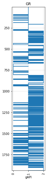
But now we’re not really dealing with regularly-sampled data anymore, we’re dealing with ‘intervals’. Striplog is sometimes a better option for representing this sort of data. So let’s try using that instead:

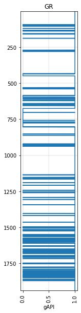
gr_blocky = gr.block(cutoffs=[40])
gr_blocky.plot()

<AxesSubplot:title={'center':'GR'}, xlabel='gAPI'>

We could find the thickest bed in this result using NumPy (i.e. the longest run of 1’s):

from itertools import groupby

samples = max(sum(run) for val, run in groupby(gr_blocky.values) if val)
samples * 0.1524

197.0532

But it’s much easier to use Striplog, which can compute the resut directly from the gr log itself. (You have to pass ‘components’ to the from_log() function, but it doesn’t matter what they are.

from striplog import Striplog

s = Striplog.from_log(gr, basis=gr.basis, cutoff=[40], components=[None, None])
s.thickest().thickness

197.05320000000017

Let’s look at how to do that with actual components…

Make a striplog instead of a blocked log#

Striplog objects are potentially a bit more versatile than trying to use a log to represent intervals.

We have to do a little extra work though; for example, we have to tell Striplog what the intervals represent… the contents (lithologies or whatever) of an interval are called ‘components’.

We also have to pass the depth separately, because Striplog doesn’t know anything about welly’s Curve objects.

from striplog import Striplog, Component

comps = [
    Component(properties={'lithology': 'sandstone'}),
    Component(properties={'lithology': 'siltstone'}),
    Component(properties={'lithology': 'shale'}),
]

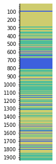
s = Striplog.from_log(gr, basis=gr.basis, cutoff=[40, 100], components=comps)

s

Striplog(853 Intervals, start=1.0668, stop=1939.1376)

You can plot this:

s.plot(aspect=3)

For a more natural visualization, it’s a good idea to make a legend to display things. For example:

from striplog import Legend

L = """comp lithology, colour, width, curve mnemonic
       sandstone, #fdf43f, 3
       siltstone, #cfbb8f, 2
       shale, #c0d0c0, 1
"""

legend = Legend.from_csv(text=L)

legend

width

component

hatch

colour

3.0

lithology

sandstone

None

#fdf43f

2.0

lithology

siltstone

None

#cfbb8f

1.0

lithology

shale

None

#c0d0c0

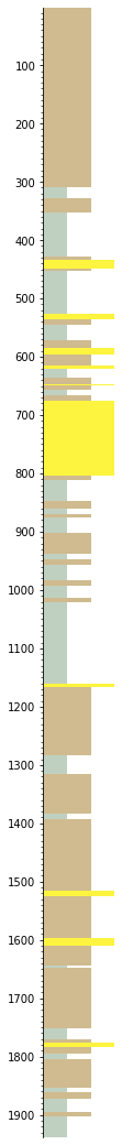
Now the plot will look more geological:

s.plot(legend=legend)

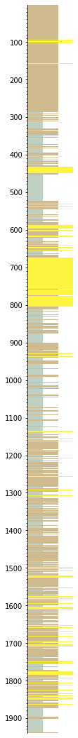
Let’s simplify it a bit by removing beds thinner than 3 m, then ‘annealing’ over the gaps, then merging like neighbours (otherwise you’ll likely have a lot of beds juxtaposed with similar beds):

s = s.prune(limit=3).anneal().merge_neighbours()

s.plot(legend=legend)

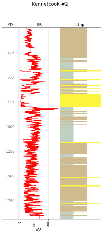
The easiest way to plot with a curve is like:

w.data['strip'] = s

tracks = ['MD', 'GR', 'strip']

C = """curve mnemonic, colour, width
       GR, #ff0000, 1
       GR-B, #ff8800, 1
"""

curve_legend = Legend.from_csv(text=C)

big_legend = legend + curve_legend

w.plot(tracks=tracks, legend=big_legend)

You can still make a blocky version from this Striplog:

gr_blocky, depth, comps = s.to_log(return_meta=True)

import matplotlib.pyplot as plt
plt.figure(figsize=(2, 10))
plt.plot(gr_blocky, depth)
plt.ylim(2000, 0)

(2000.0, 0.0)

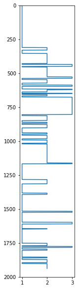
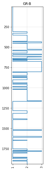
Note that this is a NumPy array, because striplog doesn’t know about welly. But you could make a welly.Curve object:

from welly import Curve

gr_blocky_curve = Curve(gr_blocky, index=depth, mnemonic='GR-B')

gr_blocky_curve.plot()

<AxesSubplot:title={'center':'GR-B'}>

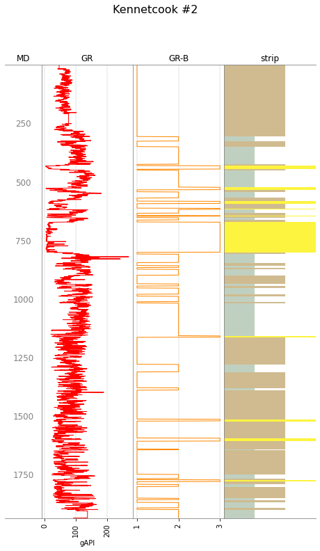
Let’s add this Curve to the well object w — then we can make a multi-track plot with welly:

w.data['GR-B'] = gr_blocky_curve

tracks = ['MD', 'GR', 'GR-B', 'strip']

w.plot(tracks=tracks, legend=big_legend)

Blocking another log using these intervals#

Let’s use the intervals we just created to block a different log from the same well.

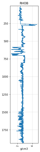
Here’s the RHOB log. We’ll block it using the intervals from the GR.

rhob = w.data['RHOB']

rhob.plot()

<AxesSubplot:title={'center':'RHOB'}, xlabel='g/cm3'>

Now we will ‘extract’ the RHOB data, using some reducing function — the default is to take the mean of the interval — into the intervals of the striplog s:

⚠️ Note that since v0.8.7 this returns a copy; before that, it worked in place.

import numpy as np

s = s.extract(rhob, basis=rhob.basis, name='RHOB', function=np.median)

Now each interval contains the mean RHOB value from that interval:

s[0]

top

1.0668

primary

lithology

siltstone

summary

308.31 m of siltstone

description

data

RHOB

2.3988199234

base

309.37199999999996

We can now turn that data ‘field’ into a log, as we did before. This time, however, we can keep the data as the value of the log — i.e. instead of having ‘bins’ from the cutoff (like 1, 2, 3, etc), we want the actual value from an interval (i.e. a density in units of g/cm³). To get this, we pass bins=False.

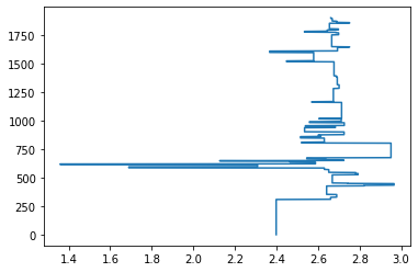
rhob_blocky, depth, _ = s.to_log(field='RHOB', bins=False, return_meta=True)

We can plot this…

plt.plot(rhob_blocky, depth)

[<matplotlib.lines.Line2D at 0x7fa9f4b1c730>]

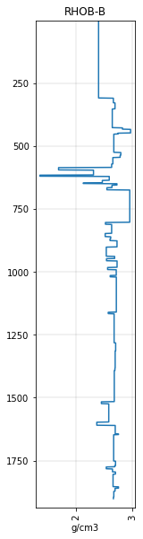
…but it’s more useful to make it into a Curve object and store it in the well object w:

rhob_blocky_curve = Curve(rhob_blocky, index=depth, mnemonic='RHOB-B', units='g/cm3')

w.data['RHOB-B'] = rhob_blocky_curve

rhob_blocky_curve.plot()

<AxesSubplot:title={'center':'RHOB-B'}, xlabel='g/cm3'>

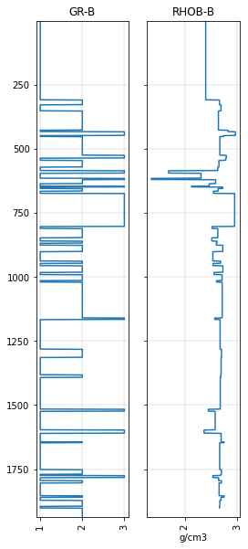
Now let’s plot it next to the blocky GR to verify that the blocks are the same:

fig, axs = plt.subplots(ncols=2, figsize=(4, 10), sharey=True)
gr_blocky_curve.plot(ax=axs[0])
rhob_blocky_curve.plot(ax=axs[1])

<AxesSubplot:title={'center':'RHOB-B'}, xlabel='g/cm3'>

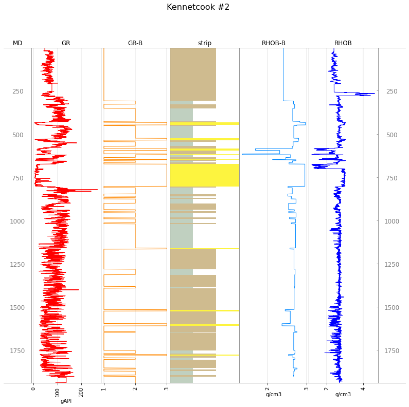
Or we can plot everything together using welly (if we first extend the legend again to accommodate the new logs):

C = """curve mnemonic, colour, width
       GR, #ff0000, 1
       GR-B, #ff8800, 1
       RHOB, #0000ff, 1
       RHOB-B, #0088ff, 1
"""

curve_legend = Legend.from_csv(text=C)

big_legend = legend + curve_legend

tracks = ['MD', 'GR', 'GR-B', 'strip', 'RHOB-B', 'RHOB', 'MD']

w.plot(tracks=tracks, legend=big_legend)