Model sequences with Markov chains#
Launch this notebook:
https://colab.research.google.com/github/agile-geoscience/striplog/blob/develop/tutorial/Markov_chains.ipynb
You need striplog version 0.8.6 or later for this notebook to work as intended.
import striplog

striplog.__version__
'unknown'
Two ways to get a Markov chain#
There are two ways to generate a Markov chain:
Parse one or more sequences of states. This will be turned into a transition matrix, from which a probability matrix will be computed.
Directly from a transition matrix, if you already have that data.
Let’s look at the transition matrix first, since that’s how Powers & Easterling presented the data in their paper on this topic.
Powers & Easterling data#
Key reference: Powers, DW and RG Easterling (1982). Improved methodology for using embedded Markov chains to describe cyclical sediments. Journal of Sedimentary Petrology 52 (3), p 913–923.
Let’s use one of the examples in Powers & Easterling — they use this transition matrix from Gingerich, PD (1969). Markov analysis of cyclic alluvial sediments. Journal of Sedimentary Petrology, 39, p. 330-332. https://doi.org/10.1306/74D71C4E-2B21-11D7-8648000102C1865D
from striplog.markov import Markov_chain
data = [[ 0, 37,  3,  2],
        [21,  0, 41, 14],
        [20, 25,  0,  0],
        [ 1, 14,  1,  0]]

m = Markov_chain(data, states=['A', 'B', 'C', 'D'])

m
Markov_chain(179 transitions, states=['A', 'B', 'C', 'D'], step=1, include_self=False)
Note that they do not include self-transitions in their data. So the elements being counted are simple ‘beds’ not ‘depth samples’ (say).
If you build a Markov chain using a matrix with self-transitions, these will be preserved; note include_self=True in the example here:
data = [[10, 37,  3,  2],
        [21, 20, 41, 14],
        [20, 25, 20,  0],
        [ 1, 14,  1, 10]]

Markov_chain(data)
Markov_chain(239 transitions, states=[0, 1, 2, 3], step=1, include_self=True)
Testing for independence#
We use the model of quasi-independence given in Powers & Easterling, as opposed to an independent model like scipy.stats.chi2_contingency(), for computing chi-squared and the expected transitions:
First, let’s look at the expected transition frequencies of the original Powers & Easterling data:
import numpy as np

np.set_printoptions(precision=3)
m.expected_counts
array([[ 0.   , 31.271,  8.171,  2.558],
       [31.282,  0.   , 34.057, 10.661],
       [ 8.171, 34.044,  0.   ,  2.785],
       [ 2.558, 10.657,  2.785,  0.   ]])
The \(\chi^2\) statistic shows the value for the observed ordering, along with the critical value at (by default) the 95% confidence level. If the first number is higher than the second number (ideally much higher), then we can reject the hypothesis that the ordering is quasi-independent. That is, we have shown that the ordering is non-random.
m.chi_squared()
Chi2(chi2=35.73687369691601, crit=11.070497693516351, perc=0.9999989278539752)
Which transitions are interesting?#
The normalized difference shows which transitions are ‘interesting’. These numbers can be interpreted as standard deviations away from the model of quasi-independence. That is, transitions with large positive numbers represent passages that occur more often than might be expected. Any numbers greater than 2 are likely to be important.
m.normalized_difference
array([[ 0.   ,  1.025, -1.809, -0.349],
       [-1.838,  0.   ,  1.19 ,  1.023],
       [ 4.138, -1.55 ,  0.   , -1.669],
       [-0.974,  1.024, -1.07 ,  0.   ]])
We can visualize this as an image:
m.plot_norm_diff()
<AxesSubplot:>
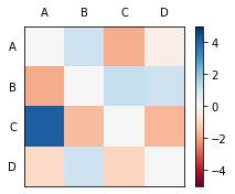
We can also interpret this matrix as a graph. The upward transitions from C to A are particularly strong in this one. Transitions from A to C happen less often than we’d expect. Those from B to D and D to B, less so.
It’s arguably easier to interpret the data when this matrix is interpreted as a directed graph:
m.plot_graph()
Please install networkx with `pip install networkx`.
We can look at an undirected version of the graph too. It downplays non-reciprocal relationships. I’m not sure this is useful…
m.plot_graph(directed=False)
Please install networkx with `pip install networkx`.
Generating random sequences#
We can generate a random succession of beds with the same transition statistics:
''.join(m.generate_states(n=30))
'ABCADBACABCBDCABDBDBCBDBABCBDB'
Again, this will respect the absence or presence of self-transitions, e.g.:
data = [[10, 37,  3,  2],
        [21, 20, 41, 14],
        [20, 25, 20,  0],
        [ 1, 14,  1, 10]]

x = Markov_chain(data)

''.join(map(str, x.generate_states(n=30)))
'112120133312110121000003122010'
Parse states#
Striplog can interpret various kinds of data as sequences of states. For example, it can get the unique elements and a ‘sequence of sequences’ from:
A simple list of states, eg
[1,2,2,2,1,1]A string of states, eg
'ABBDDDDDCCCC'A list of lists of states, eg
[[1,2,2,3], [2,4,2]](NB, not same length)A list of strings of states, eg
['aaabb', 'aabbccc'](NB, not same length)A list of state names, eg
['sst', 'mud', 'sst'](requires optional argument)A list of lists of state names, eg
[['SS', 'M', 'SS'], ['M', 'M', 'LS']]
The corresponding sets of unique states look like:
[1, 2]['A', 'B', 'C', 'D'][1, 2, 3, 4]['a', 'b', 'c']['mud', sst']['LS', 'M', 'SS']
Let’s look at a data example…
Data from Matt’s thesis#
These are the transitions from some measured sections in my PhD thesis. They start at the bottom, so in Log 7, we start with lithofacies 1 (offshore mudstone) and pass upwards into lithofacies 3, then back into 1, then 3, and so on.
We can instantiate a Markov_chain object from a sequence using its from_sequence() method. This expects either a sequence of ‘states’ (numbers or letters or strings representing rock types) or a sequence of sequences of states.
data = {
    'log7':  [1, 3, 1, 3, 5, 1, 2, 1, 3, 1, 5, 6, 1, 2, 1, 2, 1, 2, 1, 3, 5, 6, 5, 1],
    'log9':  [1, 3, 1, 5, 1, 5, 3, 1, 2, 1, 2, 1, 3, 5, 1, 5, 6, 5, 6, 1, 2, 1, 5, 6, 1],
    'log11': [1, 3, 1, 2, 1, 5, 3, 1, 2, 1, 2, 1, 3, 5, 3, 5, 1, 9, 5, 5, 5, 5, 6, 1],
    'log12': [1, 5, 3, 1, 2, 1, 2, 1, 2, 1, 4, 5, 6, 1, 2, 1, 4, 5, 1, 5, 5, 5, 1, 2, 1, 8, 9, 10, 9, 5, 1],
    'log13': [1, 6, 1, 3, 1, 3, 5, 3, 6, 1, 6, 5, 3, 1, 5, 1, 2, 1, 4, 3, 5, 3, 4, 3, 5, 1, 5, 9, 11, 9, 1],
    'log14': [1, 3, 1, 5, 8, 5, 6, 1, 3, 4, 5, 3, 1, 3, 5, 1, 7, 7, 7, 1, 7, 1, 3, 8, 5, 5, 1, 5, 9, 9, 11, 9, 1],
    'log15': [1, 8, 1, 3, 5, 1, 2, 3, 6, 3, 6, 5, 2, 1, 2, 1, 8, 5, 1, 5, 9, 9, 11, 1],
    'log16': [1, 8, 1, 5, 1, 5, 5, 6, 1, 3, 5, 3, 5, 5, 5, 8, 5, 1, 9, 9, 3, 1],
    'log17': [1, 3, 8, 1, 8, 5, 1, 8, 9, 5, 10, 5, 8, 9, 10, 8, 5, 1, 8, 9, 1],
    'log18': [1, 8, 2, 1, 2, 1, 10, 8, 9, 5, 5, 1, 2, 1, 2, 9, 5, 9, 5, 8, 5, 9, 1]
}

logs = list(data.values())

m = Markov_chain.from_sequence(logs)
m.states
array([ 1, 2, 3, 4, 5, 6, 7, 8, 9, 10, 11])
m.observed_counts
array([[ 0, 21, 17,  3, 15,  2,  2,  8,  2,  1,  0],
       [21,  0,  1,  0,  0,  0,  0,  0,  1,  0,  0],
       [12,  0,  0,  2, 12,  3,  0,  2,  0,  0,  0],
       [ 0,  0,  2,  0,  3,  0,  0,  0,  0,  0,  0],
       [19,  1,  9,  0,  0,  9,  0,  4,  5,  1,  0],
       [ 9,  0,  1,  0,  4,  0,  0,  0,  0,  0,  0],
       [ 2,  0,  0,  0,  0,  0,  0,  0,  0,  0,  0],
       [ 3,  1,  0,  0,  7,  0,  0,  0,  5,  0,  0],
       [ 4,  0,  1,  0,  6,  0,  0,  0,  0,  2,  3],
       [ 0,  0,  0,  0,  1,  0,  0,  2,  1,  0,  0],
       [ 1,  0,  0,  0,  0,  0,  0,  0,  2,  0,  0]])
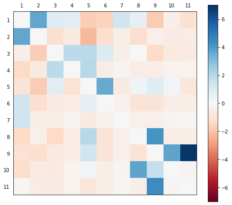
Let’s check out the normalized difference matrix:
m.expected_counts
array([[0.000e+00, 9.734e+00, 1.362e+01, 1.972e+00, 2.329e+01, 5.709e+00,
        7.807e-01, 6.576e+00, 6.576e+00, 1.572e+00, 1.175e+00],
       [9.734e+00, 0.000e+00, 2.949e+00, 4.270e-01, 5.042e+00, 1.236e+00,
        1.690e-01, 1.424e+00, 1.424e+00, 3.404e-01, 2.544e-01],
       [1.362e+01, 2.949e+00, 0.000e+00, 5.974e-01, 7.054e+00, 1.729e+00,
        2.365e-01, 1.992e+00, 1.992e+00, 4.762e-01, 3.559e-01],
       [1.972e+00, 4.270e-01, 5.974e-01, 0.000e+00, 1.022e+00, 2.504e-01,
        3.425e-02, 2.885e-01, 2.885e-01, 6.896e-02, 5.154e-02],
       [2.329e+01, 5.042e+00, 7.054e+00, 1.021e+00, 0.000e+00, 2.957e+00,
        4.044e-01, 3.406e+00, 3.406e+00, 8.143e-01, 6.086e-01],
       [5.709e+00, 1.236e+00, 1.729e+00, 2.504e-01, 2.957e+00, 0.000e+00,
        9.914e-02, 8.351e-01, 8.351e-01, 1.996e-01, 1.492e-01],
       [7.806e-01, 1.690e-01, 2.365e-01, 3.425e-02, 4.044e-01, 9.914e-02,
        0.000e+00, 1.142e-01, 1.142e-01, 2.730e-02, 2.040e-02],
       [6.576e+00, 1.424e+00, 1.992e+00, 2.885e-01, 3.406e+00, 8.351e-01,
        1.142e-01, 0.000e+00, 9.620e-01, 2.300e-01, 1.719e-01],
       [6.576e+00, 1.424e+00, 1.992e+00, 2.885e-01, 3.406e+00, 8.351e-01,
        1.142e-01, 9.620e-01, 0.000e+00, 2.300e-01, 1.719e-01],
       [1.572e+00, 3.404e-01, 4.762e-01, 6.896e-02, 8.143e-01, 1.996e-01,
        2.730e-02, 2.300e-01, 2.300e-01, 0.000e+00, 4.109e-02],
       [1.175e+00, 2.544e-01, 3.559e-01, 5.154e-02, 6.086e-01, 1.492e-01,
        2.040e-02, 1.719e-01, 1.719e-01, 4.109e-02, 0.000e+00]])
It’s hard to read this but we can change NumPy’s display options:
np.set_printoptions(suppress=True, precision=1, linewidth=120)
m.normalized_difference
array([[ 0. ,  3.6,  0.9,  0.7, -1.7, -1.6,  1.4,  0.6, -1.8, -0.5, -1.1],
       [ 3.6,  0. , -1.1, -0.7, -2.2, -1.1, -0.4, -1.2, -0.4, -0.6, -0.5],
       [-0.4, -1.7,  0. ,  1.8,  1.9,  1. , -0.5,  0. , -1.4, -0.7, -0.6],
       [-1.4, -0.7,  1.8,  0. ,  2. , -0.5, -0.2, -0.5, -0.5, -0.3, -0.2],
       [-0.9, -1.8,  0.7, -1. ,  0. ,  3.5, -0.6,  0.3,  0.9,  0.2, -0.8],
       [ 1.4, -1.1, -0.6, -0.5,  0.6,  0. , -0.3, -0.9, -0.9, -0.4, -0.4],
       [ 1.4, -0.4, -0.5, -0.2, -0.6, -0.3,  0. , -0.3, -0.3, -0.2, -0.1],
       [-1.4, -0.4, -1.4, -0.5,  1.9, -0.9, -0.3,  0. ,  4.1, -0.5, -0.4],
       [-1. , -1.2, -0.7, -0.5,  1.4, -0.9, -0.3, -1. ,  0. ,  3.7,  6.8],
       [-1.3, -0.6, -0.7, -0.3,  0.2, -0.4, -0.2,  3.7,  1.6,  0. , -0.2],
       [-0.2, -0.5, -0.6, -0.2, -0.8, -0.4, -0.1, -0.4,  4.4, -0.2,  0. ]])
Or use a graphical view:
m.plot_norm_diff()
<AxesSubplot:>
And the graph version. Note you can re-run this cell to rearrange the graph.
m.plot_graph(figsize=(15,15), max_size=2400, edge_labels=True, seed=13)
Please install networkx with `pip install networkx`.
Experimental implementation!
Multistep Markov chains are a bit of an experiment in `striplog`. Please [get in touch](mailto:matt@agilescientific.com) if you have thoughts about how it should work.
Multistep transitions#
Step = 2#
So far we’ve just been looking at direct this-to-that transitions, i.e. only considering each previous transition. What if we use the previous-but-one?
m = Markov_chain.from_sequence(logs, step=2)
m
Markov_chain(213 transitions, states=[1, 2, 3, 4, 5, 6, 7, 8, 9, 10, 11], step=2, include_self=False)
Note that self-transitions are ignored by default. With multi-step transitions, this results in a lot of zeros because we don’t just eliminate transitions like 1 > 1 > 1, but also 1 > 1 > 2 and 1 > 1 > 3, etc, as well as 1 > 2 > 2, 1 > 3 > 3, etc, and 2 > 1 > 1, 3 > 1 > 1, etc. (But we will keep 1 > 2 > 1.)
Now we have a 3D array of transition probabilities.
m.normalized_difference.shape
(11, 11, 11)
This is hard to inspect! Let’s just get the indices of the highest values.
If we add one to the indices, we’ll have a handy list of facies number transitions, since these are just 1 to 11. So we can interpret these as transitions with anomalously high probability.

There are 11 × 11 × 11 = 1331 transitions in this array (inluding self-transitions).
cutoff = 5  # 1.96 is 95% confidence

idx = np.where(m.normalized_difference > cutoff)
locs = np.array(list(zip(*idx)))

scores = {tuple(loc+1):score for score, loc in zip(m.normalized_difference[idx], locs)}

for (a, b, c), score in sorted(scores.items(), key=lambda pair: pair[1], reverse=True):
    print(f"{a:<2} -> {b:<2} -> {c:<2}   {score:.3f}")
9  -> 11 -> 9    14.602
7  -> 1  -> 7    12.685
10 -> 8  -> 9    12.685
1  -> 2  -> 1    10.109
8  -> 9  -> 10   9.441
2  -> 1  -> 2    8.542
11 -> 9  -> 1    7.825
9  -> 10 -> 8    6.676
2  -> 1  -> 4    5.864
9  -> 10 -> 9    5.851
5  -> 6  -> 1    5.372
m.chi_squared()
Chi2(chi2=1425.2383461290872, crit=112.02198574980785, perc=1.0)
Unfortunately, it’s a bit harder to draw this as a graph. Technically, it’s a hypergraph.
# This should error for now.
# m.plot_graph(figsize=(15,15), max_size=2400, edge_labels=True)
Also, the expected counts or frequencies are a bit… hard to interpret:
np.set_printoptions(suppress=True, precision=3, linewidth=120)

m.expected_counts
array([[[0.   , 0.   , 0.   , ..., 0.   , 0.   , 0.   ],
        [2.624, 0.   , 1.197, ..., 0.681, 0.141, 0.16 ],
        [3.484, 1.323, 0.   , ..., 0.792, 0.221, 0.184],
        ...,
        [1.851, 0.574, 0.869, ..., 0.   , 0.16 , 0.098],
        [0.411, 0.172, 0.273, ..., 0.12 , 0.   , 0.018],
        [0.384, 0.15 , 0.135, ..., 0.077, 0.031, 0.   ]],

       [[0.   , 0.899, 1.252, ..., 0.632, 0.16 , 0.123],
        [0.   , 0.   , 0.   , ..., 0.   , 0.   , 0.   ],
        [1.311, 0.399, 0.   , ..., 0.233, 0.055, 0.043],
        ...,
        [0.638, 0.249, 0.304, ..., 0.   , 0.049, 0.031],
        [0.15 , 0.043, 0.086, ..., 0.031, 0.   , 0.003],
        [0.15 , 0.061, 0.046, ..., 0.028, 0.006, 0.   ]],

       [[0.   , 1.215, 1.722, ..., 0.918, 0.221, 0.178],
        [1.258, 0.   , 0.556, ..., 0.215, 0.058, 0.071],
        [0.   , 0.   , 0.   , ..., 0.   , 0.   , 0.   ],
        ...,
        [0.826, 0.316, 0.384, ..., 0.   , 0.068, 0.049],
        [0.181, 0.068, 0.092, ..., 0.064, 0.   , 0.012],
        [0.163, 0.049, 0.077, ..., 0.037, 0.009, 0.   ]],

       ...,

       [[0.   , 0.611, 0.816, ..., 0.396, 0.12 , 0.08 ],
        [0.632, 0.   , 0.319, ..., 0.15 , 0.025, 0.037],
        [0.936, 0.289, 0.   , ..., 0.196, 0.046, 0.043],
        ...,
        [0.   , 0.   , 0.   , ..., 0.   , 0.   , 0.   ],
        [0.15 , 0.04 , 0.074, ..., 0.028, 0.   , 0.003],
        [0.126, 0.015, 0.043, ..., 0.018, 0.009, 0.   ]],

       [[0.   , 0.153, 0.166, ..., 0.101, 0.015, 0.018],
        [0.187, 0.   , 0.071, ..., 0.028, 0.009, 0.009],
        [0.246, 0.068, 0.   , ..., 0.052, 0.009, 0.009],
        ...,
        [0.129, 0.058, 0.061, ..., 0.   , 0.   , 0.009],
        [0.   , 0.   , 0.   , ..., 0.   , 0.   , 0.   ],
        [0.025, 0.015, 0.006, ..., 0.006, 0.   , 0.   ]],

       [[0.   , 0.135, 0.15 , ..., 0.086, 0.018, 0.018],
        [0.117, 0.   , 0.055, ..., 0.031, 0.006, 0.006],
        [0.144, 0.052, 0.   , ..., 0.04 , 0.012, 0.006],
        ...,
        [0.061, 0.034, 0.034, ..., 0.   , 0.   , 0.003],
        [0.028, 0.003, 0.012, ..., 0.009, 0.   , 0.   ],
        [0.   , 0.   , 0.   , ..., 0.   , 0.   , 0.   ]]])
Step = 3#
We can actually make a model for any number of steps, but we will need commensurately more data, especially if we’re not going to include self-transitions:
m = Markov_chain.from_sequence(logs, step=3)
m
Markov_chain(193 transitions, states=[1, 2, 3, 4, 5, 6, 7, 8, 9, 10, 11], step=3, include_self=False)
I have no idea how to visualize or interpret this thing, let me know if you do something with it!
From Striplog() instance#
I use striplog to represent stratigraphy. Let’s make a Markov chain model from an instance of striplog!
First, we’ll make a striplog by applying a couple of cut-offs to a GR log:
from welly import Well
from striplog import Striplog, Component

w = Well.from_las("P-129_out.LAS")
gr = w.data['GR']

comps = [Component({'lithology': 'sandstone'}),
         Component({'lithology': 'greywacke'}),
         Component({'lithology': 'shale'}),
        ]

s = Striplog.from_log(gr, cutoff=[30, 90], components=comps, basis=gr.basis)
s
Striplog(672 Intervals, start=1.0668, stop=1939.1376)
s.plot()
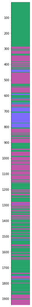
Here’s what one bed (interval in striplog’s vocabulary) looks like:
s[0]
| top | 1.0668 | ||
| primary |
| ||
| summary | 135.79 m of greywacke | ||
| description | |||
| data | |||
| base | 136.8552 |
It’s easy to get the ‘lithology’ attribute from all the beds:
seq = [i.primary.lithology for i in s]
This is what we need!
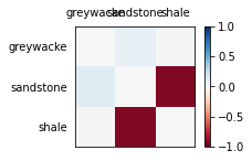
m = Markov_chain.from_sequence(seq, strings_are_states=True, include_self=False)
m.normalized_difference
array([[ 0.   ,  0.085,  0.023],
       [ 0.121,  0.   , -0.926],
       [-0.008, -0.928,  0.   ]])
m.plot_norm_diff()
<AxesSubplot:>
m.plot_graph()
Please install networkx with `pip install networkx`.
© Agile Scientific 2020, licensed CC-BY / Apache 2.0, please share this work