Extract curves into striplogs#
Sometimes you’d like to summarize or otherwise extract curve data (e.g. wireline log data) into a striplog (e.g. one that represents formations).
We’ll start by making some fake CSV text — we’ll make 5 formations called A, B, C, D and E:
data = """Comp Formation,Depth
A,100
B,200
C,250
D,400
E,600"""
If you have a CSV file, you can do:
s = Striplog.from_csv(filename=filename)
But we have text, so we do something slightly different, passing the text argument instead. We also pass a stop argument to tell Striplog to make the last unit (E) 50 m thick. (If you don’t do this, it will be 1 m thick).
from striplog import Striplog

s = Striplog.from_csv(text=data, stop=650)
/opt/hostedtoolcache/Python/3.10.4/x64/lib/python3.10/site-packages/striplog/striplog.py:512: UserWarning: No lexicon provided, using the default.
  warnings.warn(w)
Each element of the striplog is an Interval object, which has a top, base and one or more Components, which represent whatever is in the interval (maybe a rock type, or in this case a formation). There is also a data field, which we will use later.
s[0]
| top | 100.0 | ||
| primary |
| ||
| summary | 100.00 m of A | ||
| description | |||
| data | |||
| base | 200.0 |
We can plot the striplog. By default, it will use a random legend for the colours:
s.plot(aspect=3)
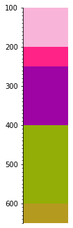
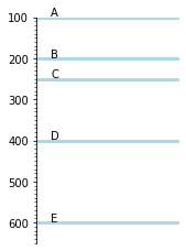
Or we can plot in the ‘tops’ style:
s.plot(style='tops', field='formation', aspect=1)
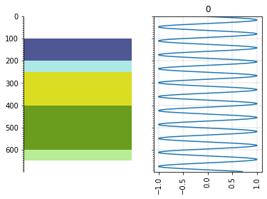
Random curve data#
Make some fake data:
from welly import Curve
import numpy as np

depth = np.linspace(0, 699, 700)
data = np.sin(depth/10)
curve = Curve(data=data, index=depth)
Plot it:
import matplotlib.pyplot as plt

fig, axs = plt.subplots(ncols=2, sharey=True)

axs[0] = s.plot(ax=axs[0])
axs[1] = curve.plot(ax=axs[1])
Extract data from the curve into the striplog#
s = s.extract(curve.values, basis=depth, name='GR')
Now we have some the GR data from each unit stored in that unit:
s[1]
| top | 200.0 | ||
| primary |
| ||
| summary | 50.00 m of B | ||
| description | |||
| data |
| ||
| base | 250.0 |
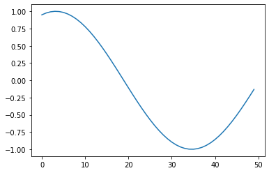
So we could plot a segment of curve, say:
plt.plot(s[1].data['GR'])
[<matplotlib.lines.Line2D at 0x7f2cfa844d60>]
Extract and reduce data#
We don’t have to store all the data points. We can optionaly pass a function to produce anything we like, and store the result of that:
s = s.extract(curve, basis=depth, name='GRmean', function=np.nanmean)

s[1]
| top | 200.0 | ||||
| primary |
| ||||
| summary | 50.00 m of B | ||||
| description | |||||
| data |
| ||||
| base | 250.0 |
Other helpful reducing functions:
np.nanmedian— median average (ignoring nans)np.product— productnp.nansum— sum (ignoring nans)np.nanmin— minimum (ignoring nans)np.nanmax— maximum (ignoring nans)scipy.stats.mstats.mode— mode averagescipy.stats.mstats.hmean— harmonic meanscipy.stats.mstats.gmean— geometric mean
Or you can write your own, for example:
def trim_mean(a):
    """Compute trimmed mean, trimming min and max"""
    return (np.nansum(a) - np.nanmin(a) - np.nanmax(a)) / a.size
Then do:
s.extract(curve, basis=basis, name='GRtrim', function=trim_mean)
The function doesn’t have to return a single number like this, it could return anything you like, including a dictionary.
We can also add bits to the data dictionary manually:
s[1].data['foo'] = 'bar'
s[1]
| top | 200.0 | ||||||
| primary |
| ||||||
| summary | 50.00 m of B | ||||||
| description | |||||||
| data |
| ||||||
| base | 250.0 |