Quick start#
This notebooks looks at the main striplog object. For the basic objects it depends on, see Basic objects.
First, import anything we might need.
import matplotlib.pyplot as plt
import numpy as np

import striplog
striplog.__version__
'unknown'
Making a striplog from CSV data#
Suppose we have CSV data like this:
csv_string = """top, base, comp lithology, comp grainsize
  230.329,  233.269,  Grey sandstone, vf-f
  233.269,  234.700,  Anhydrite,
  234.700,  236.596,  Dolomite,
  236.596,  237.911,  Red siltstone,
  237.911,  238.723,  Anhydrite,
  238.723,  239.807,  Grey sandstone, vf-f
  239.807,  240.774,  Red siltstone,
  240.774,  241.122,  Dolomite,
  241.122,  241.702,  Grey siltstone,
  241.702,  243.095,  Dolomite,
"""
Because the lithology column is named comp lithology (or component lithology), striplog will interpret this column as the lithology of a component. Likewise, the grainsize is pulled out as another property. However, the colour of the rock is not pulled out – it remains combined with the lithology.
from striplog import Striplog

strip = Striplog.from_csv(text=csv_string)
/opt/hostedtoolcache/Python/3.10.4/x64/lib/python3.10/site-packages/striplog/striplog.py:512: UserWarning: No lexicon provided, using the default.
  warnings.warn(w)
strip.plot(aspect=3)
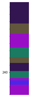
Later we’ll see how to make this plot look nicer.
Let’s look at one interval of the striplog. We’ll choose the first one, because it has the grainsize property. It looks like this:
strip[0]
| top | 230.329 | ||||
| primary |
| ||||
| summary | 2.94 m of Grey sandstone, vf-f | ||||
| description | |||||
| data | |||||
| base | 233.269 |
Adding a lexicon#
Often, we don’t have properties conveniently separated out into columns like the example above. Instead we have data like:
Light grey vf sandstone
We can get striplog to pull these different properties apart for us, by using a Lexicon. This is a dictionary-like look-up table that tells Striplog what different words mean. For example, using the default lexicon, here are the things it understands to be ‘lithologies’:
from striplog import Lexicon

lexicon = Lexicon.default()

lexicon.lithology
['overburden',
 'sandstone',
 'siltstone',
 'shale',
 'conglomerate',
 'mudstone',
 'limestone',
 'dolomite',
 'salt',
 'halite',
 'anhydrite',
 'gypsum',
 'sylvite',
 'clay',
 'mud',
 'silt',
 'sand',
 'gravel',
 'boulders']
And grainsize (these use regular expressions to capture variance in how grainsize might be expressed; all of them are case insensitive):
lexicon.grainsize
['vf(?:-)?',
 'f(?:-)?',
 'm(?:-)?',
 'c(?:-)?',
 'vc',
 'very fine(?: to)?',
 'fine(?: to)?',
 'medium(?: to)?',
 'coarse(?: to)?',
 'very coarse',
 'v fine(?: to)?',
 'med(?: to)?',
 'med.(?: to)?',
 'v coarse',
 'grains?',
 'granules?',
 'pebbles?',
 'cobbles?',
 'boulders?']
Now we can accept data in which the descriptions combine several properties:
csv_string = """top, base, description
  200.000,  230.329,  Anhydrite
  230.329,  233.269,  Grey vf-f sandstone
  233.269,  234.700,  Anhydrite
  234.700,  236.596,  Dolomite
  236.596,  237.911,  Red siltstone
  237.911,  238.723,  Anhydrite
  238.723,  239.807,  Grey vf-f sandstone
  239.807,  240.774,  Red siltstone
  240.774,  241.122,  Dolomite
  241.122,  241.702,  Grey siltstone
  241.702,  243.095,  Dolomite
  243.095,  246.654,  Grey vf-f sandstone
  246.654,  247.234,  Dolomite
  247.234,  255.435,  Grey vf-f sandstone
  255.435,  258.723,  Grey siltstone
  258.723,  259.729,  Dolomite
  259.729,  260.967,  Grey siltstone
  260.967,  261.354,  Dolomite
  261.354,  267.041,  Grey siltstone
  267.041,  267.350,  Dolomite
  267.350,  274.004,  Grey siltstone
  274.004,  274.313,  Dolomite
  274.313,  294.816,  Grey siltstone
  294.816,  295.397,  Dolomite
  295.397,  296.286,  Limestone
  296.286,  300.000,  Volcanic
"""
Let’s see how the lexicon parses one of these ‘descriptions’:
from striplog import Component

Component.from_text('Light grey vf-f sandstone', lexicon)
| lithology | sandstone |
| grainsize | vf-f |
| colour | light grey |
Now we can pass in the CSV text and apply the lexicon to it, producing a striplog:
strip2 = Striplog.from_csv(text=csv_string, lexicon=lexicon, )
strip2
Striplog(26 Intervals, start=200.0, stop=300.0)
strip2[1]
| top | 230.329 | ||||||
| primary |
| ||||||
| summary | 2.94 m of sandstone, vf-f, grey | ||||||
| description | Grey vf-f sandstone | ||||||
| data | |||||||
| base | 233.269 |
Making a striplog from an image#
We originally made striplog for a specific use-case: we had a lot of images of striplogs, with tops and bottom depths. So striplog can read images and try to make striplog objects out of them:
Here is one of the images we will convert into striplogs:

imgfile = "M-MG-70_14.3_135.9.png"
Striplog’s Legend class maps ‘components’ (rocks, if you will) to display styles (colour, width, etc). We will eventually use a legend to control how striplogs are displayed, but a legend can also control how a striplog image is interpreted.
from striplog import Legend

legend = Legend.builtin('NSDOE')
strip = Striplog.from_image(imgfile, 14.3, 135.9, legend=legend)
strip
Striplog(26 Intervals, start=14.3, stop=135.9)
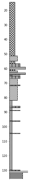
strip.plot(legend, ladder=True, aspect=5)
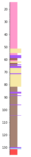
This thing might look like the image (because it uses the same legend), but it’s data:
strip[0]
| top | 14.3 | ||
| primary |
| ||
| summary | 36.94 m of anhydrite | ||
| description | |||
| data | |||
| base | 51.24117647058824 |
Representations of a striplog#
There are several ways to inspect a striplog:
printprints the contents of the striploguniqueshows us a list of the primary lithologies in the striplog, in order of cumulative thicknesshistogrammakes a histogram of the lithologies (and also returns the histogram data)plotmakes a plot of the striplog with coloured bars
print(strip[:5])
{'top': Position({'middle': 14.3, 'units': 'm'}), 'base': Position({'middle': 51.24117647058824, 'units': 'm'}), 'description': '', 'data': {}, 'components': [Component({'lithology': 'anhydrite'})]}
{'top': Position({'middle': 51.24117647058824, 'units': 'm'}), 'base': Position({'middle': 54.81764705882354, 'units': 'm'}), 'description': '', 'data': {}, 'components': [Component({'lithology': 'sandstone', 'colour': 'grey', 'grainsize': 'vf-f'})]}
{'top': Position({'middle': 54.81764705882354, 'units': 'm'}), 'base': Position({'middle': 56.55882352941177, 'units': 'm'}), 'description': '', 'data': {}, 'components': [Component({'lithology': 'anhydrite'})]}
{'top': Position({'middle': 56.55882352941177, 'units': 'm'}), 'base': Position({'middle': 58.86470588235295, 'units': 'm'}), 'description': '', 'data': {}, 'components': [Component({'lithology': 'dolomite'})]}
{'top': Position({'middle': 58.86470588235295, 'units': 'm'}), 'base': Position({'middle': 60.464705882352945, 'units': 'm'}), 'description': '', 'data': {}, 'components': [Component({'lithology': 'siltstone', 'colour': 'red'})]}
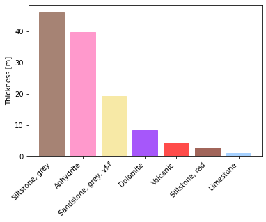
strip.unique
[(Component({'lithology': 'siltstone', 'colour': 'grey'}), 46.16470588235293),
 (Component({'lithology': 'anhydrite'}), 39.67058823529412),
 (Component({'lithology': 'sandstone', 'colour': 'grey', 'grainsize': 'vf-f'}),
  19.200000000000003),
 (Component({'lithology': 'dolomite'}), 8.282352941176498),
 (Component({'lithology': 'volcanic'}), 4.42352941176469),
 (Component({'lithology': 'siltstone', 'colour': 'red'}), 2.7764705882352843),
 (Component({'lithology': 'limestone'}), 1.082352941176481)]
_ = strip.histogram(legend=legend, rotation=45, ha='right')
You have already seen some basic plotting. For more control, you can pass some parameters to the Striplog.plot() method, but all of them are optional.
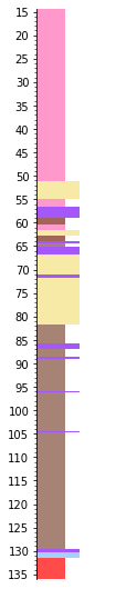
strip.plot(legend, ladder=True, aspect=5, ticks=5)
hashy_csv = """colour,width,hatch,component colour,component grainsize,component lithology
#dddddd,1,---,grey,,siltstone,
#dddddd,2,xxx,,,anhydrite,
#dddddd,3,...,grey,vf-f,sandstone,
#dddddd,4,+--,,,dolomite,
#dddddd,5,ooo,,,volcanic,
#dddddd,6,---,red,,siltstone,
#dddddd,7,,,,limestone,
"""
hashy = Legend.from_csv(text=hashy_csv)
strip.plot(hashy, ladder=True, aspect=6, lw=1)
Manipulating a striplog#
Again, the object is indexable and iterable.
print(strip[:3])
{'top': Position({'middle': 14.3, 'units': 'm'}), 'base': Position({'middle': 51.24117647058824, 'units': 'm'}), 'description': '', 'data': {}, 'components': [Component({'lithology': 'anhydrite'})]}
{'top': Position({'middle': 51.24117647058824, 'units': 'm'}), 'base': Position({'middle': 54.81764705882354, 'units': 'm'}), 'description': '', 'data': {}, 'components': [Component({'lithology': 'sandstone', 'colour': 'grey', 'grainsize': 'vf-f'})]}
{'top': Position({'middle': 54.81764705882354, 'units': 'm'}), 'base': Position({'middle': 56.55882352941177, 'units': 'm'}), 'description': '', 'data': {}, 'components': [Component({'lithology': 'anhydrite'})]}
print(strip[-1].primary.summary())
Volcanic
for i in strip[:5]:
    print(i.summary())
36.94 m of anhydrite
3.58 m of sandstone, grey, vf-f
1.74 m of anhydrite
2.31 m of dolomite
1.60 m of siltstone, red
import numpy as np

np.array([d.top.z for d in strip[5:13]])
array([60.46470588, 61.45294118, 62.77058824, 63.94705882, 64.37058824,
       65.07647059, 66.77058824, 71.1       ])
Slicing returns a new striplog:
strip[1:3]
Striplog(2 Intervals, start=51.24117647058824, stop=56.55882352941177)
You can even index into it with an iterable, like a list of indices. The result is a striplog.
indices = [2,4,6]
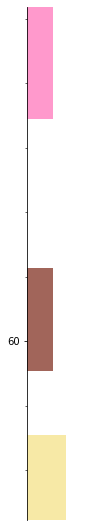
strip[indices].plot(legend, aspect=5)
You can add striplogs:
strip[:5] + strip[-5:]
Striplog(10 Intervals, start=14.3, stop=135.9)
Striplog from LAS data#
Suppose we have LAS 3.0 data like this:
las3 = """~Lithology_Parameter
LITH .                    : Lithology source          {S}
LITHD.   MD               : Lithology depth reference {S}

~Lithology_Definition
LITHT.M                   : Lithology top depth       {F}
LITHB.M                   : Lithology base depth      {F}
LITHN.                    : Lithology name            {S}

~Lithology_Data | Lithology_Definition
  200.000,  230.329,  Anhydrite
  230.329,  233.269,  Grey vf-f sandstone
  233.269,  234.700,  Anhydrite
  234.700,  236.596,  Dolomite
  236.596,  237.911,  Red siltstone
  237.911,  238.723,  Anhydrite
  238.723,  239.807,  Grey vf-f sandstone
  239.807,  240.774,  Red siltstone
  240.774,  241.122,  Dolomite
  241.122,  241.702,  Grey siltstone
  241.702,  243.095,  Dolomite
  243.095,  246.654,  Grey vf-f sandstone
  246.654,  247.234,  Dolomite
  247.234,  255.435,  Grey vf-f sandstone
  255.435,  258.723,  Grey siltstone
  258.723,  259.729,  Dolomite
  259.729,  260.967,  Grey siltstone
  260.967,  261.354,  Dolomite
  261.354,  267.041,  Grey siltstone
  267.041,  267.350,  Dolomite
  267.350,  274.004,  Grey siltstone
  274.004,  274.313,  Dolomite
  274.313,  294.816,  Grey siltstone
  294.816,  295.397,  Dolomite
  295.397,  296.286,  Limestone
  296.286,  300.000,  Volcanic
"""
There is a method for this format:
strip3 = Striplog.from_las3(las3, lexicon)
strip3
Striplog(26 Intervals, start=200.0, stop=300.0)
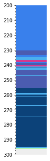
strip3.plot(aspect=3)
We can also produce a file like this from a striplog:
print(strip3.to_las3())
~Lithology_Parameter
LITH .   Striplog         : Lithology source          {S}
LITHD.   MD               : Lithology depth reference {S}

~Lithology_Definition
LITHT.M                   : Lithology top depth       {F}
LITHB.M                   : Lithology base depth      {F}
LITHD.                    : Lithology description     {S}

~Lithology_Data | Lithology_Definition
200.0,230.329,Anhydrite
230.329,233.269,"Sandstone, vf-f, grey"
233.269,234.7,Anhydrite
234.7,236.596,Dolomite
236.596,237.911,"Siltstone, red"
237.911,238.723,Anhydrite
238.723,239.807,"Sandstone, vf-f, grey"
239.807,240.774,"Siltstone, red"
240.774,241.122,Dolomite
241.122,241.702,"Siltstone, grey"
241.702,243.095,Dolomite
243.095,246.654,"Sandstone, vf-f, grey"
246.654,247.234,Dolomite
247.234,255.435,"Sandstone, vf-f, grey"
255.435,258.723,"Siltstone, grey"
258.723,259.729,Dolomite
259.729,260.967,"Siltstone, grey"
260.967,261.354,Dolomite
261.354,267.041,"Siltstone, grey"
267.041,267.35,Dolomite
267.35,274.004,"Siltstone, grey"
274.004,274.313,Dolomite
274.313,294.816,"Siltstone, grey"
294.816,295.397,Dolomite
295.397,296.286,Limestone
296.286,300.0,
©2022 Agile Geoscience. Licensed CC-BY. striplog.py