Wells
Wells are one of the fundamental objects in welly.
Well objects include collections of Curve objects. Multiple Well objects can be stored in a Project.
On this page, we take a closer look at the Well.
First, some preliminaries…
import numpy as np
import matplotlib.pyplot as plt

import welly
welly.__version__
'0.5.3rc1'
Load a well from LAS
In the Quick Start guide you saw how to quickly create a Project from a well with:
import welly
project = welly.from_las('path/to/well.las')
A welly.Project is a collection of welly.Well objects. But if you only have a single well, you may not need a Project; a Well object on its own will do. Then you could do this:
well, = welly.from_las('path/to/well.las')
The presence of the comma after well unpacks the single item into the welly variable. (This is a Python trick, it’s not a Welly thing.)
Alternatively, you can use the Well.from_las() method to load a well by passing a filename as a str. This is really just a wrapper for lasio but instantiates a Header, Curves, etc.
from welly import Well

p129 = Well.from_las('https://geocomp.s3.amazonaws.com/data/P-129.LAS')
p129
---------------------------------------------------------------------------
HTTPError                                 Traceback (most recent call last)
File /opt/hostedtoolcache/Python/3.12.8/x64/lib/python3.12/site-packages/welly/las.py:485, in file_from_url(url)
    484 try:
--> 485     text_file = StringIO(request.urlopen(url).read().decode())
    486 except error.HTTPError as e:

File /opt/hostedtoolcache/Python/3.12.8/x64/lib/python3.12/urllib/request.py:215, in urlopen(url, data, timeout, cafile, capath, cadefault, context)
    214     opener = _opener
--> 215 return opener.open(url, data, timeout)

File /opt/hostedtoolcache/Python/3.12.8/x64/lib/python3.12/urllib/request.py:521, in OpenerDirector.open(self, fullurl, data, timeout)
    520     meth = getattr(processor, meth_name)
--> 521     response = meth(req, response)
    523 return response

File /opt/hostedtoolcache/Python/3.12.8/x64/lib/python3.12/urllib/request.py:630, in HTTPErrorProcessor.http_response(self, request, response)
    629 if not (200 <= code < 300):
--> 630     response = self.parent.error(
    631         'http', request, response, code, msg, hdrs)
    633 return response

File /opt/hostedtoolcache/Python/3.12.8/x64/lib/python3.12/urllib/request.py:559, in OpenerDirector.error(self, proto, *args)
    558 args = (dict, 'default', 'http_error_default') + orig_args
--> 559 return self._call_chain(*args)

File /opt/hostedtoolcache/Python/3.12.8/x64/lib/python3.12/urllib/request.py:492, in OpenerDirector._call_chain(self, chain, kind, meth_name, *args)
    491 func = getattr(handler, meth_name)
--> 492 result = func(*args)
    493 if result is not None:

File /opt/hostedtoolcache/Python/3.12.8/x64/lib/python3.12/urllib/request.py:639, in HTTPDefaultErrorHandler.http_error_default(self, req, fp, code, msg, hdrs)
    638 def http_error_default(self, req, fp, code, msg, hdrs):
--> 639     raise HTTPError(req.full_url, code, msg, hdrs, fp)

HTTPError: HTTP Error 403: Forbidden

During handling of the above exception, another exception occurred:

Exception                                 Traceback (most recent call last)
Cell In[2], line 3
      1 from welly import Well
----> 3 p129 = Well.from_las('https://geocomp.s3.amazonaws.com/data/P-129.LAS')
      4 p129

File /opt/hostedtoolcache/Python/3.12.8/x64/lib/python3.12/site-packages/welly/well.py:303, in Well.from_las(cls, fname, remap, funcs, data, req, alias, encoding, printfname, index, **kwargs)
    301 # If https URL is passed try reading and formatting it to text file.
    302 if re.match(r'https?://.+\..+/.+?', fname) is not None:
--> 303     fname = file_from_url(fname)
    305 datasets = from_las(fname, encoding=encoding, **kwargs)
    307 # Create well from datasets.

File /opt/hostedtoolcache/Python/3.12.8/x64/lib/python3.12/site-packages/welly/las.py:487, in file_from_url(url)
    485     text_file = StringIO(request.urlopen(url).read().decode())
    486 except error.HTTPError as e:
--> 487     raise Exception('Could not retrieve url: ', e)
    489 return text_file

Exception: ('Could not retrieve url: ', <HTTPError 403: 'Forbidden'>)
There are a lot of problems here:
The Location is not stored correctly, with latitude stored in Location and Longitude stored in UWI (that’s why it appears in the title row of this view).
There’s less accurate Lat and Lon information stored in Section and Township; we should get rid of those.
There’s no UWI, KB or TD, all of which would be useful to populate.
We can fix all this by ‘remapping’ some fields. This is done with a dictionary that maps a well’s field to its location in the LAS file. For example, we can use the Well field (‘Kennetcook #2’) to as the UWI in our well with a mapping like: {'UWI': 'WELL'}. We can remove a bad item such as the Section name, by mapping to None:
remap = {
    'UWI': 'LIC',  # Commonly used unique name; not a true UWI.
    'KB': 'EKB',
    'TD': 'TDD',  # Driller's TD.
    'LATI': 'LOC',
    'LONG': 'UWI',
    'SECT': None,
    'TOWN': None,
    'LOC': None
}

p129 = Well.from_las('https://geocomp.s3.amazonaws.com/data/P-129.LAS', remap=remap)
p129
Only engine='normal' can read wrapped files
| Kennetcook #2 P-129 | |
|---|---|
| crs | CRS({}) |
| country | CA |
| province | Nova Scotia |
| latitude | Lat = 45* 12' 34.237" N |
| longitude | Long = 63* 45'24.460 W |
| datum | |
| range | PD 176 |
| ekb | 94.8 |
| egl | 90.3 |
| kb | 94.8 |
| gl | 90.3 |
| td | 1935.0 |
| tdd | 1935.0 |
| tdl | 1935.0 |
| data | CALI, DPHI_DOL, DPHI_LIM, DPHI_SAN, DRHO, DT, DTS, GR, HCAL, NPHI_DOL, NPHI_LIM, NPHI_SAN, PEF, RHOB, RLA1, RLA2, RLA3, RLA4, RLA5, RM_HRLT, RT_HRLT, RXOZ, RXO_HRLT, SP |
That’s better!
Later on, we’ll look at how we can go a step further, extracting the more accurate
Well header
Metadata about the well is stored in its header attribute:
p129.header
| original_mnemonic | mnemonic | unit | value | descr | section | |
|---|---|---|---|---|---|---|
| 0 | VERS | VERS | 2.0 | Version | ||
| 1 | WRAP | WRAP | YES | Version | ||
| 2 | STRT | STRT | M | 1.0668 | START DEPTH | Well |
| 3 | STOP | STOP | M | 1939.1376 | STOP DEPTH | Well |
| 4 | STEP | STEP | M | 0.1524 | STEP | Well |
| ... | ... | ... | ... | ... | ... | ... |
| 137 | TLI | TLI | M | 280.0 | Top Log Interval | Parameter |
| 138 | UWID | UWID | Unique Well Identification Number | Parameter | ||
| 139 | WN | WN | Kennetcook #2 | Well Name | Parameter | |
| 140 | EPD | EPD | M | 90.300003 | Elevation of Permanent Datum above Mean Sea Level | Parameter |
| 141 | UNKNOWN | Other |
142 rows × 6 columns
Important note
At present, the well’s header contains a DataFrame with the entire LAS file header.
In a future release, only the well information from the WELL part of the file will be stored in the well’s header. (The Params data goes into the well.location attribute, and the Curve data goes into Welly’s Curve objects.)
Well location
The well’s location contains the location info from PARAMS, and will also store the well’s 3D positional information, if available.
p129.location
Location({'position': None, 'crs': CRS({}), 'country': 'CA', 'province': 'Nova Scotia', 'latitude': 'Lat = 45* 12\' 34.237" N', 'longitude': "Long = 63* 45'24.460 W", 'datum': '', 'range': 'PD 176', 'ekb': 94.8, 'egl': 90.3, 'kb': 94.8, 'gl': 90.3, 'td': 1935.0, 'tdd': 1935.0, 'tdl': 1935.0, 'deviation': None})
The CRS for this well is missing; we can add one if we know it:
p129.location.crs = welly.CRS.from_epsg(2038)

p129.location
Location({'position': None, 'crs': CRS({'init': 'epsg:2038', 'no_defs': True}), 'country': 'CA', 'province': 'Nova Scotia', 'latitude': 'Lat = 45* 12\' 34.237" N', 'longitude': "Long = 63* 45'24.460 W", 'datum': '', 'range': 'PD 176', 'ekb': 94.8, 'egl': 90.3, 'kb': 94.8, 'gl': 90.3, 'td': 1935.0, 'tdd': 1935.0, 'tdl': 1935.0, 'deviation': None})
Right now there’s no position log — we need to load a deviation survey.
p129.location.position
Add deviation data to a well
Let’s load another well:
import numpy as np
from welly import Well

p130 = Well.from_las('https://geocomp.s3.amazonaws.com/data/P-130.LAS')

dev = np.loadtxt('https://geocomp.s3.amazonaws.com/data/P-130_deviation_survey.csv',
                 delimiter=',', skiprows=1
                )
The columns are MD, inclination, azimuth, and TVD.
dev[:5]
array([[ 18. ,   0.3,   0. ,  18. ],
       [ 38. ,   0.5,   0. ,  38. ],
       [ 57. ,   1.5,   0. ,  57. ],
       [ 84. ,   1.8,   0. ,  84. ],
       [104. ,   0.5,   0. , 104. ]])
add_deviation wants only MD, inclination and azimuth, in that order. Given an array like that, it computes a position log.
p130.location.add_deviation(dev[:, :3], td=2618.3)
The columns in the position log are x offset, y offset, and TVD.
p130.location.position[:5]
array([[0.00000000e+00, 0.00000000e+00, 0.00000000e+00],
       [0.00000000e+00, 4.71237821e-02, 1.79999178e+01],
       [0.00000000e+00, 1.86748917e-01, 3.79994202e+01],
       [0.00000000e+00, 5.18340431e-01, 5.69962853e+01],
       [0.00000000e+00, 1.29577626e+00, 8.39850594e+01]])
p130.location.trajectory()
array([[ 6.45933639e-01,  3.47023772e-01, -1.65395432e-02],
       [ 5.90396925e-01,  3.28218888e-01, -2.63643779e+00],
       [ 5.36457735e-01,  3.11968468e-01, -5.25632568e+00],
       ...,
       [-3.68094384e+00,  3.97484953e+01, -2.61112780e+03],
       [-3.68832058e+00,  3.96833189e+01, -2.61374906e+03],
       [-3.69619567e+00,  3.96172858e+01, -2.61637033e+03]])
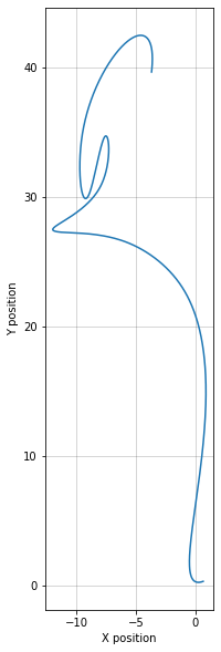
p130.location.plot_plan()
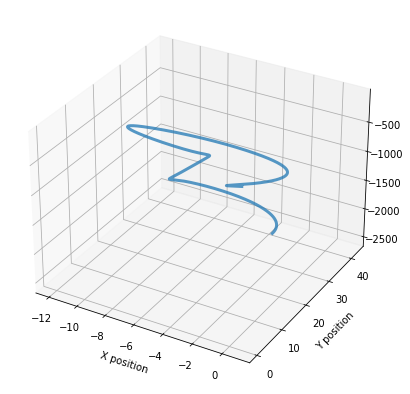
p130.location.plot_3d()
Quick plot
welly produces matplotlib plots easily… but they aren’t all that pretty. You can pass in an Axes object as ax, and you can embellish the plots by adding more matplotlib commands.
First, let’s do the simplest thing possible:
p130.plot()
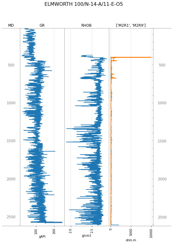
Since we have a position log, it’s worth plotting TVD as well (though it’s almost the same as MD in this well).
tracks = ['MD', 'GR', 'RHOB', ['M2R1', 'M2R9'], 'TVD']

p130.plot(tracks=tracks)
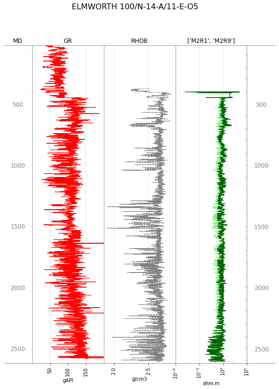
You can control the plotting style, but it requires a striplog.Legend. We find the easiest way to build one is with a CSV-like text string:
from striplog import Legend

curve_legend_csv = """curve mnemonic, colour,    lw,  ls,    xlim, xscale
                      GR,             #ff0000,   1.0,  -, "0,200", linear
                      RHOB,           gray,      1.0, --,        , linear
                      M2R9,           darkgreen, 1.0,  -,        , log
                      M2R1,           lightgreen,1.0,  -,        , log
"""
legend = Legend.from_csv(text=curve_legend_csv)

tracks = ['MD', 'GR', 'RHOB', ['M2R1', 'M2R9'], 'TVD']

p130.plot(tracks=tracks, legend=legend)
Export curves to data matrix
Make a NumPy array out of the Curves in the well:
p130.data_as_matrix()
/home/matt/miniconda3/envs/welly/lib/python3.9/site-packages/welly/well.py:1094: UserWarning: In the next release, return_meta will be True by default. Set it to False to suppress this message. Set it to True to start using this feature now.
  warnings.warn(message)
array([[nan, nan, nan, ..., nan, nan, nan],
       [nan, nan, nan, ..., nan, nan, nan],
       [nan, nan, nan, ..., nan, nan, nan],
       ...,
       [nan, nan, nan, ..., nan, nan, nan],
       [nan, nan, nan, ..., nan, nan, nan],
       [nan, nan, nan, ..., nan, nan, nan]])
You can use aliases here, and it’s helpful to know which curve is which. You can also start and stop at new depths, to cut out the NaNs:
alias = {'Gamma': ['GRC', 'GR', 'GRX'],
         'Density': ['RHOZ', 'RHOB'],
        }

X, depth, features = p130.data_as_matrix(keys=['Gamma', 'Density', 'DT'],
                                         alias=alias,
                                         start=1200, step=1,
                                         return_meta=True
                                        )
X.shape
(2624, 3)
depth
array([1200., 1201., 1202., ..., 3821., 3822., 3823.])
features
['Gamma', 'Density', 'DT']
Export curves to pandas
You can always get the curve data as a DataFrame. The depth will be the index:
df = p130.df()
df.head()
| CALI | DT | NPHI_SAN | NPHI_LIM | NPHI_DOL | DPHI_LIM | DPHI_SAN | DPHI_DOL | M2R9 | M2R6 | M2R3 | M2R2 | M2R1 | GR | SP | PEF | DRHO | RHOB | |
|---|---|---|---|---|---|---|---|---|---|---|---|---|---|---|---|---|---|---|
| DEPT | ||||||||||||||||||
| 20.1 | NaN | NaN | NaN | NaN | NaN | NaN | NaN | NaN | NaN | NaN | NaN | NaN | NaN | NaN | NaN | NaN | NaN | NaN |
| 20.2 | NaN | NaN | NaN | NaN | NaN | NaN | NaN | NaN | NaN | NaN | NaN | NaN | NaN | NaN | NaN | NaN | NaN | NaN |
| 20.3 | NaN | NaN | NaN | NaN | NaN | NaN | NaN | NaN | NaN | NaN | NaN | NaN | NaN | NaN | NaN | NaN | NaN | NaN |
| 20.4 | NaN | NaN | NaN | NaN | NaN | NaN | NaN | NaN | NaN | NaN | NaN | NaN | NaN | NaN | NaN | NaN | NaN | NaN |
| 20.5 | NaN | NaN | NaN | NaN | NaN | NaN | NaN | NaN | NaN | NaN | NaN | NaN | NaN | NaN | NaN | NaN | NaN | NaN |
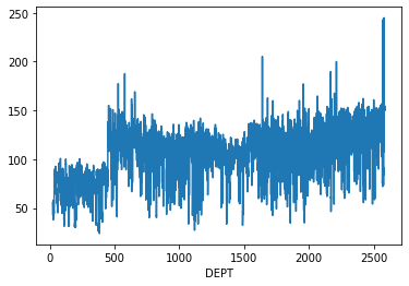
df.GR.plot()
<AxesSubplot:xlabel='DEPT'>
To get the UWI of the well as well, e.g. if you want to combine multiple wells:
df = p130.df(uwi=True)

df.head()
| CALI | DT | NPHI_SAN | NPHI_LIM | NPHI_DOL | DPHI_LIM | DPHI_SAN | DPHI_DOL | M2R9 | M2R6 | M2R3 | M2R2 | M2R1 | GR | SP | PEF | DRHO | RHOB | ||
|---|---|---|---|---|---|---|---|---|---|---|---|---|---|---|---|---|---|---|---|
| UWI | DEPT | ||||||||||||||||||
| 100/N14A/11E05 | 20.1 | NaN | NaN | NaN | NaN | NaN | NaN | NaN | NaN | NaN | NaN | NaN | NaN | NaN | NaN | NaN | NaN | NaN | NaN |
| 20.2 | NaN | NaN | NaN | NaN | NaN | NaN | NaN | NaN | NaN | NaN | NaN | NaN | NaN | NaN | NaN | NaN | NaN | NaN | |
| 20.3 | NaN | NaN | NaN | NaN | NaN | NaN | NaN | NaN | NaN | NaN | NaN | NaN | NaN | NaN | NaN | NaN | NaN | NaN | |
| 20.4 | NaN | NaN | NaN | NaN | NaN | NaN | NaN | NaN | NaN | NaN | NaN | NaN | NaN | NaN | NaN | NaN | NaN | NaN | |
| 20.5 | NaN | NaN | NaN | NaN | NaN | NaN | NaN | NaN | NaN | NaN | NaN | NaN | NaN | NaN | NaN | NaN | NaN | NaN |
If you have several wells, you can also use welly.Project.df() to do the concatenation for you.
Note that you can also use aliases with the DataFrame creation, or create a new ‘basis’ (depth in this case):
keys = ['CALI', 'Gamma', 'Density']
df = p130.df(keys=keys, alias=alias, rename_aliased=True)
df.head()
| CALI | Gamma | Density | |
|---|---|---|---|
| DEPT | |||
| 20.1 | NaN | NaN | NaN |
| 20.2 | NaN | NaN | NaN |
| 20.3 | NaN | NaN | NaN |
| 20.4 | NaN | NaN | NaN |
| 20.5 | NaN | NaN | NaN |
Make an ‘empty’ well
import welly

w = welly.Well()

w.header  # is empty
| original_mnemonic | mnemonic | unit | value | descr | section |
|---|
We can set the UWI and name of a well directly on the well object, but these are the only attributes of the well we can set in this way.
w.uwi = 'foo'
w.uwi
'foo'
w.header
| original_mnemonic | mnemonic | unit | value | descr | section | |
|---|---|---|---|---|---|---|
| 0 | UWI | UWI | None | foo | None | header |
© 2022 Agile Scientific, CC BY