Quick start
Welcome to the Quick start guide! This should help you get started using welly.
First some preliminaries…
import numpy as np
import matplotlib.pyplot as plt

import welly
welly.__version__
'0.5.3rc1'
Create a project from LAS
Use the read_las() function to load a well by passing a single filename, a POSIX-style path with wildcards (e.g. 'file_*.las') or URL as a str.
This creates a project containing one (or more, depending on the wildcard) wells.
project = welly.read_las('https://geocomp.s3.amazonaws.com/data/P-129.LAS')

project
0it [00:00, ?it/s]
0it [00:00, ?it/s]
---------------------------------------------------------------------------
HTTPError                                 Traceback (most recent call last)
File /opt/hostedtoolcache/Python/3.12.8/x64/lib/python3.12/site-packages/welly/las.py:485, in file_from_url(url)
    484 try:
--> 485     text_file = StringIO(request.urlopen(url).read().decode())
    486 except error.HTTPError as e:

File /opt/hostedtoolcache/Python/3.12.8/x64/lib/python3.12/urllib/request.py:215, in urlopen(url, data, timeout, cafile, capath, cadefault, context)
    214     opener = _opener
--> 215 return opener.open(url, data, timeout)

File /opt/hostedtoolcache/Python/3.12.8/x64/lib/python3.12/urllib/request.py:521, in OpenerDirector.open(self, fullurl, data, timeout)
    520     meth = getattr(processor, meth_name)
--> 521     response = meth(req, response)
    523 return response

File /opt/hostedtoolcache/Python/3.12.8/x64/lib/python3.12/urllib/request.py:630, in HTTPErrorProcessor.http_response(self, request, response)
    629 if not (200 <= code < 300):
--> 630     response = self.parent.error(
    631         'http', request, response, code, msg, hdrs)
    633 return response

File /opt/hostedtoolcache/Python/3.12.8/x64/lib/python3.12/urllib/request.py:559, in OpenerDirector.error(self, proto, *args)
    558 args = (dict, 'default', 'http_error_default') + orig_args
--> 559 return self._call_chain(*args)

File /opt/hostedtoolcache/Python/3.12.8/x64/lib/python3.12/urllib/request.py:492, in OpenerDirector._call_chain(self, chain, kind, meth_name, *args)
    491 func = getattr(handler, meth_name)
--> 492 result = func(*args)
    493 if result is not None:

File /opt/hostedtoolcache/Python/3.12.8/x64/lib/python3.12/urllib/request.py:639, in HTTPDefaultErrorHandler.http_error_default(self, req, fp, code, msg, hdrs)
    638 def http_error_default(self, req, fp, code, msg, hdrs):
--> 639     raise HTTPError(req.full_url, code, msg, hdrs, fp)

HTTPError: HTTP Error 403: Forbidden

During handling of the above exception, another exception occurred:

Exception                                 Traceback (most recent call last)
Cell In[2], line 1
----> 1 project = welly.read_las('https://geocomp.s3.amazonaws.com/data/P-129.LAS')
      3 project

File /opt/hostedtoolcache/Python/3.12.8/x64/lib/python3.12/site-packages/welly/__init__.py:34, in read_las(path, **kwargs)
     20 def read_las(path, **kwargs):
     21     """
     22     A package namespace method to be called as `welly.read_las`.
     23
   (...)
     32         welly.Project. The Project object.
     33     """
---> 34     return Project.from_las(path, **kwargs)

File /opt/hostedtoolcache/Python/3.12.8/x64/lib/python3.12/site-packages/welly/project.py:183, in Project.from_las(cls, path, remap, funcs, data, req, alias, max, encoding, printfname, index, **kwargs)
    180 else:
    181     uris = path  # It's a list-like of files and/or URLs.
--> 183 wells = [Well.from_las(f,
    184                        remap=remap,
    185                        funcs=funcs,
    186                        data=data,
    187                        req=req,
    188                        alias=alias,
    189                        encoding=encoding,
    190                        printfname=printfname,
    191                        index=index,
    192                        **kwargs,
    193                        )
    194          for i, f in tqdm(enumerate(uris)) if i < max]
    196 return cls(list(filter(None, wells)))

File /opt/hostedtoolcache/Python/3.12.8/x64/lib/python3.12/site-packages/welly/well.py:303, in Well.from_las(cls, fname, remap, funcs, data, req, alias, encoding, printfname, index, **kwargs)
    301 # If https URL is passed try reading and formatting it to text file.
    302 if re.match(r'https?://.+\..+/.+?', fname) is not None:
--> 303     fname = file_from_url(fname)
    305 datasets = from_las(fname, encoding=encoding, **kwargs)
    307 # Create well from datasets.

File /opt/hostedtoolcache/Python/3.12.8/x64/lib/python3.12/site-packages/welly/las.py:487, in file_from_url(url)
    485     text_file = StringIO(request.urlopen(url).read().decode())
    486 except error.HTTPError as e:
--> 487     raise Exception('Could not retrieve url: ', e)
    489 return text_file

Exception: ('Could not retrieve url: ', <HTTPError 403: 'Forbidden'>)
Clearly there are some issues with this well. Have a look at the Well object docs to see how to fix them.
You can index into a project to get at a single well.
well = project[0]

well
| Kennetcook #2 Long = 63* 45'24.460 W | |
|---|---|
| crs | CRS({}) |
| location | Lat = 45* 12' 34.237" N |
| country | CA |
| province | Nova Scotia |
| latitude | |
| longitude | |
| datum | |
| section | 45.20 Deg N |
| range | PD 176 |
| township | 63.75 Deg W |
| ekb | 94.8 |
| egl | 90.3 |
| gl | 90.3 |
| tdd | 1935.0 |
| tdl | 1935.0 |
| td | None |
| data | CALI, DPHI_DOL, DPHI_LIM, DPHI_SAN, DRHO, DT, DTS, GR, HCAL, NPHI_DOL, NPHI_LIM, NPHI_SAN, PEF, RHOB, RLA1, RLA2, RLA3, RLA4, RLA5, RM_HRLT, RT_HRLT, RXOZ, RXO_HRLT, SP |
The well’s header contains the well information from the WELL part of the file.
PLEASE NOTE The header attribute is under active development and will change in the next release of welly. We will make it more natural to find basic information about the well, without having to know how to read an LAS file.
well.header
| original_mnemonic | mnemonic | unit | value | descr | section | |
|---|---|---|---|---|---|---|
| 0 | VERS | VERS | 2.0 | Version | ||
| 1 | WRAP | WRAP | YES | Version | ||
| 2 | STRT | STRT | M | 1.0668 | START DEPTH | Well |
| 3 | STOP | STOP | M | 1939.1376 | STOP DEPTH | Well |
| 4 | STEP | STEP | M | 0.1524 | STEP | Well |
| ... | ... | ... | ... | ... | ... | ... |
| 137 | TLI | TLI | M | 280.0 | Top Log Interval | Parameter |
| 138 | UWID | UWID | Unique Well Identification Number | Parameter | ||
| 139 | WN | WN | Kennetcook #2 | Well Name | Parameter | |
| 140 | EPD | EPD | M | 90.300003 | Elevation of Permanent Datum above Mean Sea Level | Parameter |
| 141 | UNKNOWN | Other |
142 rows × 6 columns
The well’s location contains the location info from PARAMS:
well.location
Location({'position': None, 'crs': CRS({}), 'location': 'Lat = 45* 12\' 34.237" N', 'country': 'CA', 'province': 'Nova Scotia', 'latitude': '', 'longitude': '', 'datum': '', 'section': '45.20 Deg N', 'range': 'PD 176', 'township': '63.75 Deg W', 'ekb': 94.8, 'egl': 90.3, 'gl': 90.3, 'tdd': 1935.0, 'tdl': 1935.0, 'td': None, 'deviation': None})
Basic plots
Welly produces simple matplotlib plots. You can add your own Matplotlib code to build on them.
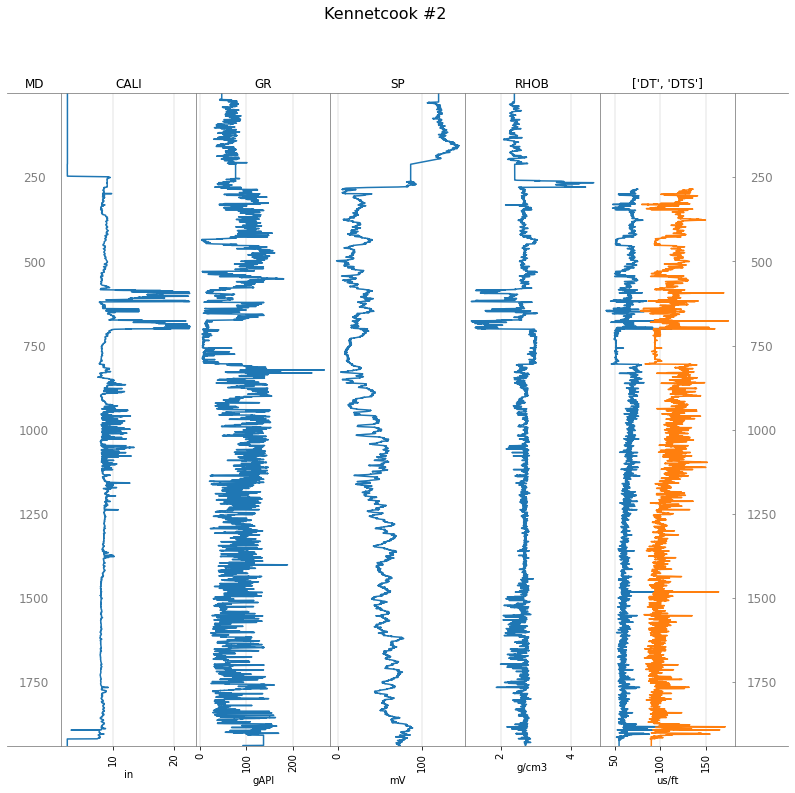
Let’s plot some important logs. We can put two logs in the same track, as shown, and add depth tracks:
tracks = ['MD', 'CALI', 'GR', 'SP', 'RHOB', ['DT', 'DTS'], 'MD']

well.plot(tracks=tracks)
Curve data
The well curves are stored in well.data, which is a dictionary mapping mnemonic to welly.Curve object:
well.data
{'CALI': Curve(mnemonic=CALI, units=in, start=1.0668, stop=1939.1376, step=0.1524, count=[12718]),
 'HCAL': Curve(mnemonic=HCAL, units=in, start=1.0668, stop=1939.1376, step=0.1524, count=[2139]),
 'PEF': Curve(mnemonic=PEF, units=, start=1.0668, stop=1939.1376, step=0.1524, count=[12718]),
 'DT': Curve(mnemonic=DT, units=us/ft, start=1.0668, stop=1939.1376, step=0.1524, count=[10850]),
 'DTS': Curve(mnemonic=DTS, units=us/ft, start=1.0668, stop=1939.1376, step=0.1524, count=[10850]),
 'DPHI_SAN': Curve(mnemonic=DPHI_SAN, units=m3/m3, start=1.0668, stop=1939.1376, step=0.1524, count=[12718]),
 'DPHI_LIM': Curve(mnemonic=DPHI_LIM, units=m3/m3, start=1.0668, stop=1939.1376, step=0.1524, count=[12718]),
 'DPHI_DOL': Curve(mnemonic=DPHI_DOL, units=m3/m3, start=1.0668, stop=1939.1376, step=0.1524, count=[12718]),
 'NPHI_SAN': Curve(mnemonic=NPHI_SAN, units=m3/m3, start=1.0668, stop=1939.1376, step=0.1524, count=[12718]),
 'NPHI_LIM': Curve(mnemonic=NPHI_LIM, units=m3/m3, start=1.0668, stop=1939.1376, step=0.1524, count=[12718]),
 'NPHI_DOL': Curve(mnemonic=NPHI_DOL, units=m3/m3, start=1.0668, stop=1939.1376, step=0.1524, count=[12718]),
 'RLA5': Curve(mnemonic=RLA5, units=ohm.m, start=1.0668, stop=1939.1376, step=0.1524, count=[12718]),
 'RLA3': Curve(mnemonic=RLA3, units=ohm.m, start=1.0668, stop=1939.1376, step=0.1524, count=[12718]),
 'RLA4': Curve(mnemonic=RLA4, units=ohm.m, start=1.0668, stop=1939.1376, step=0.1524, count=[12718]),
 'RLA1': Curve(mnemonic=RLA1, units=ohm.m, start=1.0668, stop=1939.1376, step=0.1524, count=[12718]),
 'RLA2': Curve(mnemonic=RLA2, units=ohm.m, start=1.0668, stop=1939.1376, step=0.1524, count=[12718]),
 'RXOZ': Curve(mnemonic=RXOZ, units=ohm.m, start=1.0668, stop=1939.1376, step=0.1524, count=[12718]),
 'RXO_HRLT': Curve(mnemonic=RXO_HRLT, units=ohm.m, start=1.0668, stop=1939.1376, step=0.1524, count=[2139]),
 'RT_HRLT': Curve(mnemonic=RT_HRLT, units=ohm.m, start=1.0668, stop=1939.1376, step=0.1524, count=[12718]),
 'RM_HRLT': Curve(mnemonic=RM_HRLT, units=ohm.m, start=1.0668, stop=1939.1376, step=0.1524, count=[12718]),
 'DRHO': Curve(mnemonic=DRHO, units=g/cm3, start=1.0668, stop=1939.1376, step=0.1524, count=[12718]),
 'RHOB': Curve(mnemonic=RHOB, units=g/cm3, start=1.0668, stop=1939.1376, step=0.1524, count=[12707]),
 'GR': Curve(mnemonic=GR, units=gAPI, start=1.0668, stop=1939.1376, step=0.1524, count=[12718]),
 'SP': Curve(mnemonic=SP, units=mV, start=1.0668, stop=1939.1376, step=0.1524, count=[12718])}
Let’s assign gr to the gamma-ray log so we can inspect it more easily:
gr = well.data['GR']

gr
| GR [gAPI] | |
|---|---|
| 1.0668 : 1939.1376 : 0.1524 | |
| index_units | m |
| code | None |
| description | Gamma-Ray |
| log_type | None |
| api | None |
| date | 10-Oct-2007 |
| null | -999.25 |
| run | 1 |
| service_company | Schlumberger |
| _alias | GR |
| Stats | |
| samples (NaNs) | 12718 (0) |
| min mean max | 3.89 78.986 267.94 |
| Depth | Value |
| 1.0668 | 46.6987 |
| 1.2192 | 46.6987 |
| 1.3716 | 46.6987 |
| ⋮ | ⋮ |
| 1938.8328 | 92.2462 |
| 1938.9852 | 92.2462 |
| 1939.1376 | 92.2462 |
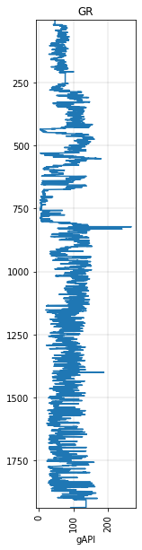
It’s often helpful to make a quick plot:
gr.plot()
<AxesSubplot:title={'center':'GR'}, xlabel='gAPI'>
Curve data as a pandas.DataFrame
The df attribute (attributes are like ordinary variables; they do not have parentheses after them) of a single curve is a dataframe:
gr.df
| GR | |
|---|---|
| DEPT | |
| 1.0668 | 46.69865036 |
| 1.2192 | 46.69865036 |
| 1.3716 | 46.69865036 |
| 1.5240 | 46.69865036 |
| 1.6764 | 46.69865036 |
| ... | ... |
| 1938.5280 | 92.24622345 |
| 1938.6804 | 92.24622345 |
| 1938.8328 | 92.24622345 |
| 1938.9852 | 92.24622345 |
| 1939.1376 | 92.24622345 |
12718 rows × 1 columns
And you can get at all of the well data in a similar way, except that this is a method not an attribute.
well.df()
| CALI | HCAL | PEF | DT | DTS | DPHI_SAN | DPHI_LIM | DPHI_DOL | NPHI_SAN | NPHI_LIM | ... | RLA1 | RLA2 | RXOZ | RXO_HRLT | RT_HRLT | RM_HRLT | DRHO | RHOB | GR | SP | |
|---|---|---|---|---|---|---|---|---|---|---|---|---|---|---|---|---|---|---|---|---|---|
| DEPT | |||||||||||||||||||||
| 1.0668 | 2.4438154697 | 4.3912849426 | 3.5864000320 | NaN | NaN | 0.1574800014 | 0.1984400004 | 0.2590999901 | 0.4650999904 | 0.3364700079 | ... | 0.0320999995 | 0.0279399995 | 0.0576100014 | 0.0255800001 | 0.0255800001 | 0.0550099984 | 0.1942329407 | 2.3901498318 | 46.69865036 | 120.1250 |
| 1.2192 | 2.4438154697 | 4.3912849426 | 3.5864000320 | NaN | NaN | 0.1574800014 | 0.1984400004 | 0.2590999901 | 0.4650999904 | 0.3364700079 | ... | 0.0320999995 | 0.0279399995 | 0.0576100014 | 0.0255800001 | 0.0255800001 | 0.0550099984 | 0.1942329407 | 2.3901498318 | 46.69865036 | 120.1250 |
| 1.3716 | 2.4438154697 | 4.3912849426 | 3.5864000320 | NaN | NaN | 0.1574800014 | 0.1984400004 | 0.2590999901 | 0.4650999904 | 0.3364700079 | ... | 0.0320999995 | 0.0279399995 | 0.0576100014 | 0.0255800001 | 0.0255800001 | 0.0550099984 | 0.1942329407 | 2.3901498318 | 46.69865036 | 120.1250 |
| 1.5240 | 2.4438154697 | 4.3912849426 | 3.5864000320 | NaN | NaN | 0.1574800014 | 0.1984400004 | 0.2590999901 | 0.4650999904 | 0.3364700079 | ... | 0.0320999995 | 0.0279399995 | 0.0576100014 | 0.0255800001 | 0.0255800001 | 0.0550099984 | 0.1942329407 | 2.3901498318 | 46.69865036 | 120.1250 |
| 1.6764 | 2.4438154697 | 4.3912849426 | 3.5864000320 | NaN | NaN | 0.1574800014 | 0.1984400004 | 0.2590999901 | 0.4650999904 | 0.3364700079 | ... | 0.0320999995 | 0.0279399995 | 0.0576100014 | 0.0255800001 | 0.0255800001 | 0.0550099984 | 0.1942329407 | 2.3901498318 | 46.69865036 | 120.1250 |
| ... | ... | ... | ... | ... | ... | ... | ... | ... | ... | ... | ... | ... | ... | ... | ... | ... | ... | ... | ... | ... | ... |
| 1938.5280 | 2.4202680588 | NaN | 2.2369799614 | NaN | NaN | 0.5464199781 | 585.9415283200 | 541.6757202100 | 0.1283400059 | 0.0841699988 | ... | 274.0264892600 | 663.1040649400 | 7.1023502350 | NaN | 7.3863301277 | 0.0272899996 | 0.0613951497 | NaN | 92.24622345 | 73.4375 |
| 1938.6804 | 2.4202680588 | NaN | 2.2369799614 | NaN | NaN | 0.5464199781 | 585.9415283200 | 541.6757202100 | 0.1283400059 | 0.0841699988 | ... | 274.0264892600 | 663.1040649400 | 7.1022100449 | NaN | 7.3860998154 | 0.0272899996 | 0.0613951497 | NaN | 92.24622345 | 73.6875 |
| 1938.8328 | 2.4202680588 | NaN | 2.2369799614 | NaN | NaN | 0.5464199781 | 585.9415283200 | 541.6757202100 | 0.1283400059 | 0.0841699988 | ... | 274.0264892600 | 663.1040649400 | 7.0968699455 | NaN | 7.3806500435 | 0.0272899996 | 0.0613951497 | NaN | 92.24622345 | 73.0000 |
| 1938.9852 | 2.4202680588 | NaN | 2.2369799614 | NaN | NaN | 0.5464199781 | 585.9415283200 | 541.6757202100 | 0.1283400059 | 0.0841699988 | ... | 274.0264892600 | 663.1040649400 | 7.0391001701 | NaN | 7.3211698532 | 0.0272899996 | 0.0613951497 | NaN | 92.24622345 | 73.9375 |
| 1939.1376 | 2.4202680588 | NaN | 2.2369799614 | NaN | NaN | 0.5464199781 | 585.9415283200 | 541.6757202100 | 0.1283400059 | 0.0841699988 | ... | 274.0264892600 | 663.1040649400 | 7.0019497871 | NaN | 7.1535902023 | 0.0272899996 | 0.0613951497 | NaN | 92.24622345 | 74.2500 |
12718 rows × 24 columns
It has to be a method because we can pass in extra options like aliases.
Curve aliases
We can make a dictionary mapping alias names (what we want to call curves) to a list of mnemonics (what they are actually called). The list of mnemonics is ordered, and this order expresses your preference. So, for example, in the alias dictionary below, the GR log will be used in preference to the GAM log.
alias = {
    "Gamma": ["GR", "GAM", "GRC", "SGR", "NGT"],
    "Density": ["RHOZ", "RHOB", "DEN", "RHOZ"],
    "Sonic": ["DT", "AC", "DTP", "DT4P"],
    "Caliper": ["CAL", "CALI", "CALS", "C1"],
    'Porosity SS': ['NPSS', 'DPSS'],
}
Lots of methods in welly take an alias. Welly will use the alias dictionary to decide what to show.
Here, the keys argument narrows down the columns to include in the dataframe.
well.df(keys=['Gamma', 'Density', 'Sonic', 'DTS'], alias=alias)
| Gamma | Density | Sonic | DTS | |
|---|---|---|---|---|
| DEPT | ||||
| 1.0668 | 46.69865036 | 2.3901498318 | NaN | NaN |
| 1.2192 | 46.69865036 | 2.3901498318 | NaN | NaN |
| 1.3716 | 46.69865036 | 2.3901498318 | NaN | NaN |
| 1.5240 | 46.69865036 | 2.3901498318 | NaN | NaN |
| 1.6764 | 46.69865036 | 2.3901498318 | NaN | NaN |
| ... | ... | ... | ... | ... |
| 1938.5280 | 92.24622345 | NaN | NaN | NaN |
| 1938.6804 | 92.24622345 | NaN | NaN | NaN |
| 1938.8328 | 92.24622345 | NaN | NaN | NaN |
| 1938.9852 | 92.24622345 | NaN | NaN | NaN |
| 1939.1376 | 92.24622345 | NaN | NaN | NaN |
12718 rows × 4 columns
There are a lot of NaNs there, but if we just wanted to see the middle of the well, we can pass in a basis to narrow it down (and even resample the data if we want).
Let’s look at 1000 to 1500 m, resampled to 1 m sample interval:
basis = range(1000, 1501)

well.df(keys=['Gamma', 'Density', 'Sonic', 'DTS'], alias=alias, basis=basis)
| Gamma | Density | Sonic | DTS | |
|---|---|---|---|---|
| DEPT | ||||
| 1.0668 | 46.69865036 | 2.3901498318 | NaN | NaN |
| 1.2192 | 46.69865036 | 2.3901498318 | NaN | NaN |
| 1.3716 | 46.69865036 | 2.3901498318 | NaN | NaN |
| 1.5240 | 46.69865036 | 2.3901498318 | NaN | NaN |
| 1.6764 | 46.69865036 | 2.3901498318 | NaN | NaN |
| ... | ... | ... | ... | ... |
| 1938.5280 | 92.24622345 | NaN | NaN | NaN |
| 1938.6804 | 92.24622345 | NaN | NaN | NaN |
| 1938.8328 | 92.24622345 | NaN | NaN | NaN |
| 1938.9852 | 92.24622345 | NaN | NaN | NaN |
| 1939.1376 | 92.24622345 | NaN | NaN | NaN |
12718 rows × 4 columns
Curve quality
We can check the quality of curves with a dictionary of tests. There are some predefined tests in the welly.quality module, but you can write your own functions and pass them in instead (the function should take a curve as its argument, and return True if the test passed).
import welly.quality as q

tests = {
    'Each': [
        q.no_flat,
        q.no_monotonic,
        q.no_gaps,
    ],
    'Gamma': [
        q.all_positive,
        q.all_below(450),
        q.check_units(['API', 'GAPI']),
    ],
    'DT': [
        q.all_positive,
    ],
    'Sonic': [
        q.all_between(1, 10000),  # 1333 to 5000 m/s
        q.no_spikes(10),          # 10 spikes allowed
    ],
}
passed = well.qc_data(tests, alias=alias)
This returns a dictionary of curves in which the values are dictionaries of test name: test result pairs.
passed
{'CALI': {'no_flat': False, 'no_monotonic': False, 'no_gaps': True},
 'HCAL': {'no_flat': False, 'no_monotonic': False, 'no_gaps': True},
 'PEF': {'no_flat': False, 'no_monotonic': False, 'no_gaps': True},
 'DT': {'no_flat': True,
  'no_monotonic': True,
  'no_gaps': True,
  'all_positive': True,
  'all_between': True,
  'no_spikes': False},
 'DTS': {'no_flat': True, 'no_monotonic': True, 'no_gaps': True},
 'DPHI_SAN': {'no_flat': False, 'no_monotonic': False, 'no_gaps': True},
 'DPHI_LIM': {'no_flat': False, 'no_monotonic': False, 'no_gaps': True},
 'DPHI_DOL': {'no_flat': False, 'no_monotonic': False, 'no_gaps': True},
 'NPHI_SAN': {'no_flat': False, 'no_monotonic': False, 'no_gaps': True},
 'NPHI_LIM': {'no_flat': False, 'no_monotonic': False, 'no_gaps': True},
 'NPHI_DOL': {'no_flat': False, 'no_monotonic': False, 'no_gaps': True},
 'RLA5': {'no_flat': False, 'no_monotonic': False, 'no_gaps': True},
 'RLA3': {'no_flat': False, 'no_monotonic': False, 'no_gaps': True},
 'RLA4': {'no_flat': False, 'no_monotonic': False, 'no_gaps': True},
 'RLA1': {'no_flat': False, 'no_monotonic': False, 'no_gaps': True},
 'RLA2': {'no_flat': False, 'no_monotonic': False, 'no_gaps': True},
 'RXOZ': {'no_flat': False, 'no_monotonic': False, 'no_gaps': True},
 'RXO_HRLT': {'no_flat': False, 'no_monotonic': False, 'no_gaps': True},
 'RT_HRLT': {'no_flat': False, 'no_monotonic': False, 'no_gaps': True},
 'RM_HRLT': {'no_flat': False, 'no_monotonic': False, 'no_gaps': True},
 'DRHO': {'no_flat': False, 'no_monotonic': False, 'no_gaps': True},
 'RHOB': {'no_flat': False, 'no_monotonic': False, 'no_gaps': True},
 'GR': {'no_flat': False,
  'no_monotonic': False,
  'no_gaps': True,
  'all_positive': True,
  'all_below': True,
  'check_units': False},
 'SP': {'no_flat': False, 'no_monotonic': False, 'no_gaps': True}}
There’s also an HTML table for rendering in Notebooks:
from IPython.display import HTML

html = well.qc_table_html(tests, alias=alias)
HTML(html)
| Curve | Passed | Score | all_below | no_flat | all_positive | no_monotonic | no_spikes | check_units | all_between | no_gaps |
|---|---|---|---|---|---|---|---|---|---|---|
| CALI | 1 / 3 | 0.333 | False | False | True | |||||
| HCAL | 1 / 3 | 0.333 | False | False | True | |||||
| PEF | 1 / 3 | 0.333 | False | False | True | |||||
| DT | 5 / 6 | 0.833 | True | True | True | False | True | True | ||
| DTS | 3 / 3 | 1.000 | True | True | True | |||||
| DPHI_SAN | 1 / 3 | 0.333 | False | False | True | |||||
| DPHI_LIM | 1 / 3 | 0.333 | False | False | True | |||||
| DPHI_DOL | 1 / 3 | 0.333 | False | False | True | |||||
| NPHI_SAN | 1 / 3 | 0.333 | False | False | True | |||||
| NPHI_LIM | 1 / 3 | 0.333 | False | False | True | |||||
| NPHI_DOL | 1 / 3 | 0.333 | False | False | True | |||||
| RLA5 | 1 / 3 | 0.333 | False | False | True | |||||
| RLA3 | 1 / 3 | 0.333 | False | False | True | |||||
| RLA4 | 1 / 3 | 0.333 | False | False | True | |||||
| RLA1 | 1 / 3 | 0.333 | False | False | True | |||||
| RLA2 | 1 / 3 | 0.333 | False | False | True | |||||
| RXOZ | 1 / 3 | 0.333 | False | False | True | |||||
| RXO_HRLT | 1 / 3 | 0.333 | False | False | True | |||||
| RT_HRLT | 1 / 3 | 0.333 | False | False | True | |||||
| RM_HRLT | 1 / 3 | 0.333 | False | False | True | |||||
| DRHO | 1 / 3 | 0.333 | False | False | True | |||||
| RHOB | 1 / 3 | 0.333 | False | False | True | |||||
| GR | 3 / 6 | 0.500 | True | False | True | False | False | True | ||
| SP | 1 / 3 | 0.333 | False | False | True |
Add a striplog
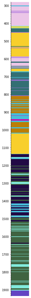
In principle, Welly can hold data from anywhere. Let’s add data from another source. Striplog can create a geological log from an image or a CSV. Let’s try it:
from striplog import Legend, Striplog

legend = Legend.builtin('NSDOE')
strip = Striplog.from_image('https://geocomp.s3.amazonaws.com/data/P-129_280_1935.png', 280, 1935, legend=legend)
strip.plot()
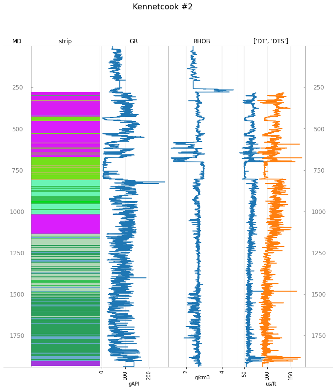
Add this to the well data:
well.data['strip'] = strip
tracks = ['MD', 'strip', 'GR', 'RHOB', ['DT', 'DTS'], 'MD']

well.plot(tracks=tracks)
Write a LAS file
At any point, you can write out a new LAS file.
Let’s write a new file with only the DT and DTS logs, and a different NULL value to the original:
well.to_las('out.las', keys=['DT', 'DTS'], null_value=-111.111)
You can perform a shell command in Jupyter Notebooks by putting a ! before the command. So on Linux, here’s how we can check the new file exists:
!ls -l out.las
-rw-rw-r-- 1 matt matt 434247 Feb 13 14:22 out.las
!head -12 out.las
~Version ---------------------------------------------------
VERS.   2.0 : CWLS log ASCII Standard -VERSION 2.0
WRAP.    NO : One line per depth step
DLM . SPACE : Column Data Section Delimiter
~Well ------------------------------------------------------
STRT  .m                    1.06680 : START DEPTH
STOP  .m                 1939.13760 : STOP DEPTH
STEP  .m                    0.15240 : STEP
NULL  .                    -111.111 : NULL VALUE
COMP  . Elmworth Energy Corporation : COMPANY
WELL  .               Kennetcook #2 : WELL
FLD   .               Windsor Block : FIELD
© 2022 Agile Scientific, CC BY