Projects
Wells are one of the fundamental objects in welly.
Well objects include collections of Curve objects. Multiple Well objects can be stored in a Project.
On this page, we take a closer look at the Project class. It lets us handle groups of wells. It is really just a list of Well objects, with a few extra powers.
First, some preliminaries…
import welly

welly.__version__
'0.5.3rc1'
Make a project
We have a few LAS files in a folder; we can load them all at once with standard POSIX file globbing syntax:
p = welly.read_las("../../tests/assets/example_*.las")
0it [00:00, ?it/s]
/opt/hostedtoolcache/Python/3.12.8/x64/lib/python3.12/site-packages/welly/curve.py:515: UserWarning: Index is not evenly sampled. Cannot derive step. Try resampling the curve with, for example `curve.to_basis(step=0.1524)`
  return get_step_from_array(self.df.index.values)
/opt/hostedtoolcache/Python/3.12.8/x64/lib/python3.12/site-packages/welly/project.py:183: UserWarning: 3-2-A: Curves have step 0. Consider reampling them with `curve.to_basis(step=0.1524)` or similar.
  wells = [Well.from_las(f,
/opt/hostedtoolcache/Python/3.12.8/x64/lib/python3.12/site-packages/welly/curve.py:515: UserWarning: Index is not evenly sampled. Cannot derive step. Try resampling the curve with, for example `curve.to_basis(step=0.1524)`
  return get_step_from_array(self.df.index.values)
/opt/hostedtoolcache/Python/3.12.8/x64/lib/python3.12/site-packages/welly/project.py:183: UserWarning: 3-2-B: Curves have step 0. Consider reampling them with `curve.to_basis(step=0.1524)` or similar.
  wells = [Well.from_las(f,

2it [00:00, 21.59it/s]
Now we have a project, containing two files:
p
| Index | UWI | Data | Curves |
|---|---|---|---|
| 0 | 3-2-A | 12 curves | SP, SN, ILD, LLS, LLD, MLL, NPHI, RHOB, CAL1, GR, DT, CAL2 |
| 1 | 3-2-B | 12 curves | SP, SN, ILD, LLS, LLD, MLL, NPHI, RHOZ, CAL1, GRC, DTP, CAL2 |
You can pass in a list of files or URLs:
p = welly.read_las(['../../tests/assets/P-129_out.LAS',
                    'https://geocomp.s3.amazonaws.com/data/P-130.LAS',
                    'https://geocomp.s3.amazonaws.com/data/R-39.las',
                   ])
0it [00:00, ?it/s]
Only engine='normal' can read wrapped files
1it [00:01, 1.37s/it]
1it [00:01, 1.61s/it]
---------------------------------------------------------------------------
HTTPError                                 Traceback (most recent call last)
File /opt/hostedtoolcache/Python/3.12.8/x64/lib/python3.12/site-packages/welly/las.py:485, in file_from_url(url)
    484 try:
--> 485     text_file = StringIO(request.urlopen(url).read().decode())
    486 except error.HTTPError as e:

File /opt/hostedtoolcache/Python/3.12.8/x64/lib/python3.12/urllib/request.py:215, in urlopen(url, data, timeout, cafile, capath, cadefault, context)
    214     opener = _opener
--> 215 return opener.open(url, data, timeout)

File /opt/hostedtoolcache/Python/3.12.8/x64/lib/python3.12/urllib/request.py:521, in OpenerDirector.open(self, fullurl, data, timeout)
    520     meth = getattr(processor, meth_name)
--> 521     response = meth(req, response)
    523 return response

File /opt/hostedtoolcache/Python/3.12.8/x64/lib/python3.12/urllib/request.py:630, in HTTPErrorProcessor.http_response(self, request, response)
    629 if not (200 <= code < 300):
--> 630     response = self.parent.error(
    631         'http', request, response, code, msg, hdrs)
    633 return response

File /opt/hostedtoolcache/Python/3.12.8/x64/lib/python3.12/urllib/request.py:559, in OpenerDirector.error(self, proto, *args)
    558 args = (dict, 'default', 'http_error_default') + orig_args
--> 559 return self._call_chain(*args)

File /opt/hostedtoolcache/Python/3.12.8/x64/lib/python3.12/urllib/request.py:492, in OpenerDirector._call_chain(self, chain, kind, meth_name, *args)
    491 func = getattr(handler, meth_name)
--> 492 result = func(*args)
    493 if result is not None:

File /opt/hostedtoolcache/Python/3.12.8/x64/lib/python3.12/urllib/request.py:639, in HTTPDefaultErrorHandler.http_error_default(self, req, fp, code, msg, hdrs)
    638 def http_error_default(self, req, fp, code, msg, hdrs):
--> 639     raise HTTPError(req.full_url, code, msg, hdrs, fp)

HTTPError: HTTP Error 403: Forbidden

During handling of the above exception, another exception occurred:

Exception                                 Traceback (most recent call last)
Cell In[4], line 1
----> 1 p = welly.read_las(['../../tests/assets/P-129_out.LAS',
      2                     'https://geocomp.s3.amazonaws.com/data/P-130.LAS',
      3                     'https://geocomp.s3.amazonaws.com/data/R-39.las',
      4                    ])

File /opt/hostedtoolcache/Python/3.12.8/x64/lib/python3.12/site-packages/welly/__init__.py:34, in read_las(path, **kwargs)
     20 def read_las(path, **kwargs):
     21     """
     22     A package namespace method to be called as `welly.read_las`.
     23
   (...)
     32         welly.Project. The Project object.
     33     """
---> 34     return Project.from_las(path, **kwargs)

File /opt/hostedtoolcache/Python/3.12.8/x64/lib/python3.12/site-packages/welly/project.py:183, in Project.from_las(cls, path, remap, funcs, data, req, alias, max, encoding, printfname, index, **kwargs)
    180 else:
    181     uris = path  # It's a list-like of files and/or URLs.
--> 183 wells = [Well.from_las(f,
    184                        remap=remap,
    185                        funcs=funcs,
    186                        data=data,
    187                        req=req,
    188                        alias=alias,
    189                        encoding=encoding,
    190                        printfname=printfname,
    191                        index=index,
    192                        **kwargs,
    193                        )
    194          for i, f in tqdm(enumerate(uris)) if i < max]
    196 return cls(list(filter(None, wells)))

File /opt/hostedtoolcache/Python/3.12.8/x64/lib/python3.12/site-packages/welly/well.py:303, in Well.from_las(cls, fname, remap, funcs, data, req, alias, encoding, printfname, index, **kwargs)
    301 # If https URL is passed try reading and formatting it to text file.
    302 if re.match(r'https?://.+\..+/.+?', fname) is not None:
--> 303     fname = file_from_url(fname)
    305 datasets = from_las(fname, encoding=encoding, **kwargs)
    307 # Create well from datasets.

File /opt/hostedtoolcache/Python/3.12.8/x64/lib/python3.12/site-packages/welly/las.py:487, in file_from_url(url)
    485     text_file = StringIO(request.urlopen(url).read().decode())
    486 except error.HTTPError as e:
--> 487     raise Exception('Could not retrieve url: ', e)
    489 return text_file

Exception: ('Could not retrieve url: ', <HTTPError 403: 'Forbidden'>)
This project has three wells:
p
| Index | UWI | Data | Curves |
|---|---|---|---|
| 0 | Long = 63* 45'24.460 W | 24 curves | CALI, HCAL, PEF, DT, DTS, DPHI_SAN, DPHI_LIM, DPHI_DOL, NPHI_SAN, NPHI_LIM, NPHI_DOL, RLA5, RLA3, RLA4, RLA1, RLA2, RXOZ, RXO_HRLT, RT_HRLT, RM_HRLT, DRHO, RHOB, GR, SP |
| 1 | 100/N14A/11E05 | 18 curves | CALI, DT, NPHI_SAN, NPHI_LIM, NPHI_DOL, DPHI_LIM, DPHI_SAN, DPHI_DOL, M2R9, M2R6, M2R3, M2R2, M2R1, GR, SP, PEF, DRHO, RHOB |
| 2 | 303N764340060300 | 22 curves | BS, CALI, CHR1, CHR2, CHRP, CHRS, DRHO, DT1R, DT2, DT2R, DT4P, DT4S, GR, HD1, HD2, HD3, NPOR, PEF, RHOB, SPR1, TENS, VPVS |
Typical, the UWIs are a disaster. Let’s ignore this for now.
The Project is really just a list-like thing, so you can index into it to get at a single well. Each well is represented by a welly.Well object.
p[0]
| Kennetcook #2 Long = 63* 45'24.460 W | |
|---|---|
| crs | CRS({}) |
| location | Lat = 45* 12' 34.237" N |
| country | CA |
| province | Nova Scotia |
| latitude | |
| longitude | |
| datum | |
| section | 45.20 Deg N |
| range | PD 176 |
| township | 63.75 Deg W |
| ekb | 94.8 |
| egl | 90.3 |
| gl | 90.3 |
| tdd | 1935.0 |
| tdl | 1935.0 |
| td | None |
| data | CALI, DPHI_DOL, DPHI_LIM, DPHI_SAN, DRHO, DT, DTS, GR, HCAL, NPHI_DOL, NPHI_LIM, NPHI_SAN, PEF, RHOB, RLA1, RLA2, RLA3, RLA4, RLA5, RM_HRLT, RT_HRLT, RXOZ, RXO_HRLT, SP |
Some of the fields of this LAS file are messed up; see the Well notebook for more on how to fix this.
Plot curves from several wells
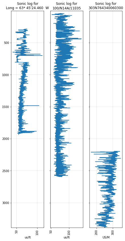
The DT log is called DT4P in one of the wells. We can deal with this sort of issue with aliases. Let’s set up an alias dictionary, then plot the DT log from each well:
alias = {'Sonic': ['DT', 'DT4P'],
         'Caliper': ['HCAL', 'CALI'],
        }
import matplotlib.pyplot as plt

fig, axs = plt.subplots(figsize=(7, 14),
                        ncols=len(p),
                        sharey=True,
                        )

for i, (ax, w) in enumerate(zip(axs, p)):
    log = w.get_curve('Sonic', alias=alias)
    if log is not None:
        ax = log.plot(ax=ax)
    ax.set_title("Sonic log for\n{}".format(w.uwi))

min_z, max_z = p.basis_range

plt.ylim(max_z, min_z)
plt.show()
Get a pandas.DataFrame
The df() method makes a DataFrame using a dual index of UWI and Depth.
Before we export our wells, let’s give Kennetcook #2 a better UWI:
p[0].uwi = p[0].name
p[0]
| Kennetcook #2 Kennetcook #2 | |
|---|---|
| crs | CRS({}) |
| location | Lat = 45* 12' 34.237" N |
| country | CA |
| province | Nova Scotia |
| latitude | |
| longitude | |
| datum | |
| section | 45.20 Deg N |
| range | PD 176 |
| township | 63.75 Deg W |
| ekb | 94.8 |
| egl | 90.3 |
| gl | 90.3 |
| tdd | 1935.0 |
| tdl | 1935.0 |
| td | None |
| data | CALI, DPHI_DOL, DPHI_LIM, DPHI_SAN, DRHO, DT, DTS, GR, HCAL, NPHI_DOL, NPHI_LIM, NPHI_SAN, PEF, RHOB, RLA1, RLA2, RLA3, RLA4, RLA5, RM_HRLT, RT_HRLT, RXOZ, RXO_HRLT, SP |
That’s better.
When creating the DataFrame, you can pass a list of the keys (mnemonics) you want, and use aliases as usual.
alias
{'Sonic': ['DT', 'DT4P'], 'Caliper': ['HCAL', 'CALI']}
keys = ['Caliper', 'GR', 'Sonic']

df = p.df(keys=keys, alias=alias, rename_aliased=True)
df
| Caliper | GR | Sonic | ||
|---|---|---|---|---|
| UWI | DEPT | |||
| Kennetcook #2 | 1.0668000000 | 4.3912849426 | 46.6986503600 | NaN |
| 1.2192000000 | 4.3912849426 | 46.6986503600 | NaN | |
| 1.3716000000 | 4.3912849426 | 46.6986503600 | NaN | |
| 1.5240000000 | 4.3912849426 | 46.6986503600 | NaN | |
| 1.6764000000 | 4.3912849426 | 46.6986503600 | NaN | |
| ... | ... | ... | ... | ... |
| 303N764340060300 | 3387.5471999996 | 303.7090000000 | 32.0276000039 | 252.4951 |
| 3387.6995999996 | 303.7090000000 | 32.0276000000 | 252.4951 | |
| 3387.8519999996 | 303.7090000000 | 32.0276000000 | 252.4951 | |
| 3388.0043999996 | 303.7090000000 | 32.0276000000 | 252.4951 | |
| 3388.1567999996 | 303.7090000000 | 32.0276000000 | 252.4951 |
46594 rows × 3 columns
Quality
Welly can run quality tests on the curves in your project. Some of the tests take arguments. You can test for things like this:
all_positive: Passes if all the values are greater than zero.all_above(50): Passes if all the values are greater than 50.mean_below(100): Passes if the mean of the log is less than 100.no_nans: Passes if there are no NaNs in the log.no_flat: Passes if there are no sections of well log with the same values (e.g. because a gap was interpolated across with a constant value).no_monotonic: Passes if there are no monotonic ramps in the log (e.g. because a gap was linearly interpolated across).
Insert lists of tests into a dictionary with any of the following key examples:
'GR': The test(s) will run against the GR log.'Gamma': The test(s) will run against the log matching according to the alias dictionary.'Each': The test(s) will run against every log in a well.'All': Some tests take multiple logs as input, for examplequality.no_similarities. These test(s) will run against all the logs as a group. Could be quite slow, because there may be a lot of pairwise comparisons to do.
The tests are run against all wells in the project. If you only want to run against a subset of the wells, make a new project for them.
import welly.quality as q

tests = {
    'All': [q.no_similarities],
    'Each': [q.no_gaps, q.no_monotonic, q.no_flat],
    'GR': [q.all_positive],
    'Sonic': [q.all_positive, q.all_between(50, 200)],
}
Let’s add our own test for units:
def has_si_units(curve):
    return curve.units.lower() in ['mm', 'gapi', 'us/m', 'k/m3']

tests['Each'].append(has_si_units)
We’ll use the same alias dictionary as before:
alias
{'Sonic': ['DT', 'DT4P'], 'Caliper': ['HCAL', 'CALI']}
Now we can run the tests and look at the results, which are in an HTML table:
from IPython.display import HTML

HTML(p.curve_table_html(keys=['Caliper', 'GR', 'Sonic', 'SP', 'RHOB'],
                        tests=tests, alias=alias)
    )
| Idx | UWI | Data | Passing | Caliper* | GR | Sonic* | SP | RHOB |
|---|---|---|---|---|---|---|---|---|
| % | 3/3 wells | 3/3 wells | 3/3 wells | 2/3 wells | 3/3 wells | |||
| 0 | Kennetcook #2 | 5/24 curves | 54 | HCAL ⬤ 4.39 in | GR ⬤ 78.99 gAPI | DT ⬤ 63.08 us/ft | SP ⬤ 52.47 mV | RHOB ⬤ 2.61 g/cm3 |
| 1 | 100/N14A/11E05 | 5/18 curves | 79 | CALI ⬤ 8.90 in | GR ⬤ 103.74 gAPI | DT ⬤ 74.90 us/ft | SP ⬤ 101.60 mV | RHOB ⬤ 2.62 g/cm3 |
| 2 | 303N764340060300 | 4/22 curves | 78 | CALI ⬤ 311.97 MM | GR ⬤ 67.49 GAPI | DT4P ⬤ 279.84 US/M | ⬤ | RHOB ⬤ 2493.56 K/M3 |
Here’s how to interpret the result:
Green background: the log is present. You can see the mean value and the units (check them!!).
Grey background: the log is not present.
And the traffic light dots (hover to see how many tests passed):
Green dot: all the tests passed.
Orange dot: some tests failed.
Red dot: all tests failed.
Grey dot: no tests ran.
The Passing percentage shows how many tests passed for that well.
© 2022 Agile Scientific, CC BY