Curves
Curves are one of the fundamental objects in welly.
Well objects include collections of Curve objects. Multiple Well objects can be stored in a Project.
On this page, we take a closer look at the Curve object.
Some preliminaries…
import numpy as np
import matplotlib.pyplot as plt

import welly
welly.__version__
'0.5.3rc1'
Load a well from LAS
Use the from_las() method to load a well by passing a filename as a str.
This is really just a wrapper for lasio but instantiates a Header, Curves, etc.
from welly import Well

p129 = Well.from_las('https://geocomp.s3.amazonaws.com/data/P-129.LAS')
---------------------------------------------------------------------------
HTTPError                                 Traceback (most recent call last)
File /opt/hostedtoolcache/Python/3.12.8/x64/lib/python3.12/site-packages/welly/las.py:485, in file_from_url(url)
    484 try:
--> 485     text_file = StringIO(request.urlopen(url).read().decode())
    486 except error.HTTPError as e:

File /opt/hostedtoolcache/Python/3.12.8/x64/lib/python3.12/urllib/request.py:215, in urlopen(url, data, timeout, cafile, capath, cadefault, context)
    214     opener = _opener
--> 215 return opener.open(url, data, timeout)

File /opt/hostedtoolcache/Python/3.12.8/x64/lib/python3.12/urllib/request.py:521, in OpenerDirector.open(self, fullurl, data, timeout)
    520     meth = getattr(processor, meth_name)
--> 521     response = meth(req, response)
    523 return response

File /opt/hostedtoolcache/Python/3.12.8/x64/lib/python3.12/urllib/request.py:630, in HTTPErrorProcessor.http_response(self, request, response)
    629 if not (200 <= code < 300):
--> 630     response = self.parent.error(
    631         'http', request, response, code, msg, hdrs)
    633 return response

File /opt/hostedtoolcache/Python/3.12.8/x64/lib/python3.12/urllib/request.py:559, in OpenerDirector.error(self, proto, *args)
    558 args = (dict, 'default', 'http_error_default') + orig_args
--> 559 return self._call_chain(*args)

File /opt/hostedtoolcache/Python/3.12.8/x64/lib/python3.12/urllib/request.py:492, in OpenerDirector._call_chain(self, chain, kind, meth_name, *args)
    491 func = getattr(handler, meth_name)
--> 492 result = func(*args)
    493 if result is not None:

File /opt/hostedtoolcache/Python/3.12.8/x64/lib/python3.12/urllib/request.py:639, in HTTPDefaultErrorHandler.http_error_default(self, req, fp, code, msg, hdrs)
    638 def http_error_default(self, req, fp, code, msg, hdrs):
--> 639     raise HTTPError(req.full_url, code, msg, hdrs, fp)

HTTPError: HTTP Error 403: Forbidden

During handling of the above exception, another exception occurred:

Exception                                 Traceback (most recent call last)
Cell In[2], line 3
      1 from welly import Well
----> 3 p129 = Well.from_las('https://geocomp.s3.amazonaws.com/data/P-129.LAS')

File /opt/hostedtoolcache/Python/3.12.8/x64/lib/python3.12/site-packages/welly/well.py:303, in Well.from_las(cls, fname, remap, funcs, data, req, alias, encoding, printfname, index, **kwargs)
    301 # If https URL is passed try reading and formatting it to text file.
    302 if re.match(r'https?://.+\..+/.+?', fname) is not None:
--> 303     fname = file_from_url(fname)
    305 datasets = from_las(fname, encoding=encoding, **kwargs)
    307 # Create well from datasets.

File /opt/hostedtoolcache/Python/3.12.8/x64/lib/python3.12/site-packages/welly/las.py:487, in file_from_url(url)
    485     text_file = StringIO(request.urlopen(url).read().decode())
    486 except error.HTTPError as e:
--> 487     raise Exception('Could not retrieve url: ', e)
    489 return text_file

Exception: ('Could not retrieve url: ', <HTTPError 403: 'Forbidden'>)
p129.plot()
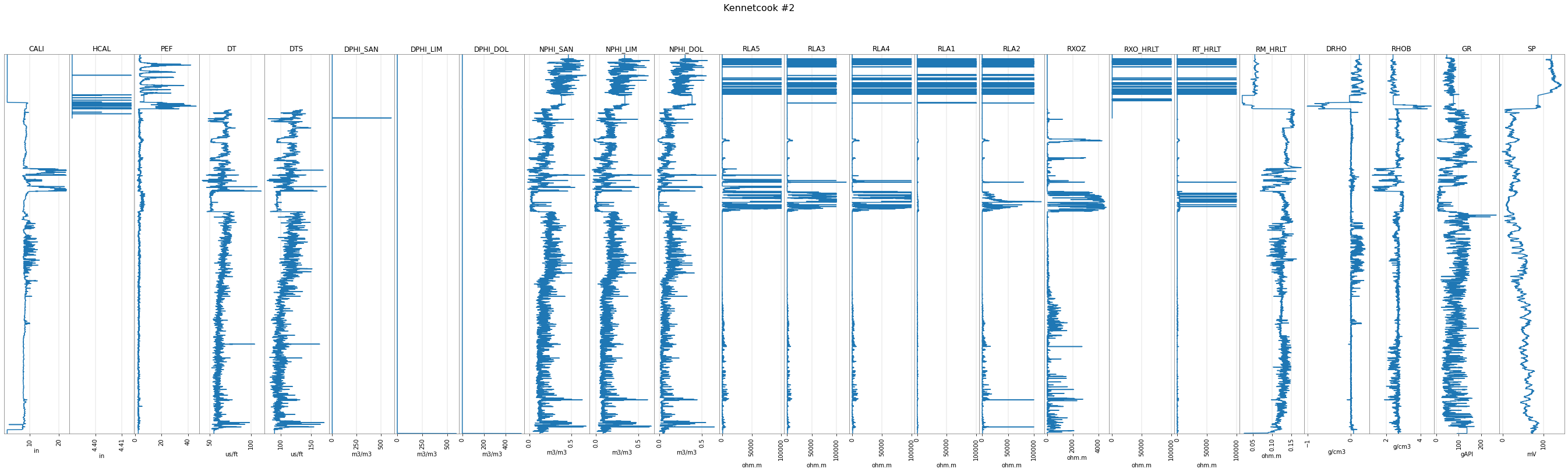
The curves are stored in the data attribute, which is an ordinary dictionary:
p129.data
{'CALI': Curve(mnemonic=CALI, units=in, start=1.0668, stop=1939.1376, step=0.1524, count=[12718]),
 'HCAL': Curve(mnemonic=HCAL, units=in, start=1.0668, stop=1939.1376, step=0.1524, count=[2139]),
 'PEF': Curve(mnemonic=PEF, units=, start=1.0668, stop=1939.1376, step=0.1524, count=[12718]),
 'DT': Curve(mnemonic=DT, units=us/ft, start=1.0668, stop=1939.1376, step=0.1524, count=[10850]),
 'DTS': Curve(mnemonic=DTS, units=us/ft, start=1.0668, stop=1939.1376, step=0.1524, count=[10850]),
 'DPHI_SAN': Curve(mnemonic=DPHI_SAN, units=m3/m3, start=1.0668, stop=1939.1376, step=0.1524, count=[12718]),
 'DPHI_LIM': Curve(mnemonic=DPHI_LIM, units=m3/m3, start=1.0668, stop=1939.1376, step=0.1524, count=[12718]),
 'DPHI_DOL': Curve(mnemonic=DPHI_DOL, units=m3/m3, start=1.0668, stop=1939.1376, step=0.1524, count=[12718]),
 'NPHI_SAN': Curve(mnemonic=NPHI_SAN, units=m3/m3, start=1.0668, stop=1939.1376, step=0.1524, count=[12718]),
 'NPHI_LIM': Curve(mnemonic=NPHI_LIM, units=m3/m3, start=1.0668, stop=1939.1376, step=0.1524, count=[12718]),
 'NPHI_DOL': Curve(mnemonic=NPHI_DOL, units=m3/m3, start=1.0668, stop=1939.1376, step=0.1524, count=[12718]),
 'RLA5': Curve(mnemonic=RLA5, units=ohm.m, start=1.0668, stop=1939.1376, step=0.1524, count=[12718]),
 'RLA3': Curve(mnemonic=RLA3, units=ohm.m, start=1.0668, stop=1939.1376, step=0.1524, count=[12718]),
 'RLA4': Curve(mnemonic=RLA4, units=ohm.m, start=1.0668, stop=1939.1376, step=0.1524, count=[12718]),
 'RLA1': Curve(mnemonic=RLA1, units=ohm.m, start=1.0668, stop=1939.1376, step=0.1524, count=[12718]),
 'RLA2': Curve(mnemonic=RLA2, units=ohm.m, start=1.0668, stop=1939.1376, step=0.1524, count=[12718]),
 'RXOZ': Curve(mnemonic=RXOZ, units=ohm.m, start=1.0668, stop=1939.1376, step=0.1524, count=[12718]),
 'RXO_HRLT': Curve(mnemonic=RXO_HRLT, units=ohm.m, start=1.0668, stop=1939.1376, step=0.1524, count=[2139]),
 'RT_HRLT': Curve(mnemonic=RT_HRLT, units=ohm.m, start=1.0668, stop=1939.1376, step=0.1524, count=[12718]),
 'RM_HRLT': Curve(mnemonic=RM_HRLT, units=ohm.m, start=1.0668, stop=1939.1376, step=0.1524, count=[12718]),
 'DRHO': Curve(mnemonic=DRHO, units=g/cm3, start=1.0668, stop=1939.1376, step=0.1524, count=[12718]),
 'RHOB': Curve(mnemonic=RHOB, units=g/cm3, start=1.0668, stop=1939.1376, step=0.1524, count=[12707]),
 'GR': Curve(mnemonic=GR, units=gAPI, start=1.0668, stop=1939.1376, step=0.1524, count=[12718]),
 'SP': Curve(mnemonic=SP, units=mV, start=1.0668, stop=1939.1376, step=0.1524, count=[12718])}
Let’s look at one log:
gr = p129.data['GR']

gr
| GR [gAPI] | |
|---|---|
| 1.0668 : 1939.1376 : 0.1524 | |
| index_units | m |
| code | None |
| description | Gamma-Ray |
| log_type | None |
| api | None |
| date | 10-Oct-2007 |
| null | -999.25 |
| run | 1 |
| service_company | Schlumberger |
| _alias | GR |
| Stats | |
| samples (NaNs) | 12718 (0) |
| min mean max | 3.89 78.986 267.94 |
| Depth | Value |
| 1.0668 | 46.6987 |
| 1.2192 | 46.6987 |
| 1.3716 | 46.6987 |
| ⋮ | ⋮ |
| 1938.8328 | 92.2462 |
| 1938.9852 | 92.2462 |
| 1939.1376 | 92.2462 |
The object knows some things about itself:
gr.mnemonic, gr.units, gr.start, gr.stop, gr.step
('GR', 'gAPI', 1.0668, 1939.1376, 0.1524000000000001)
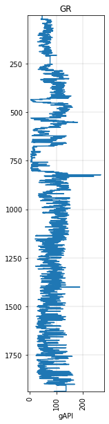
Curves have various methods on them, such as plot()…
gr.plot()
<AxesSubplot:title={'center':'GR'}, xlabel='gAPI'>
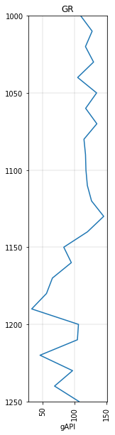
Often we just want to look at or deal with a portion of the curve, or maybe resample it:
gr.to_basis(start=1000, stop=1250, step=10.0).plot()
<AxesSubplot:title={'center':'GR'}, xlabel='gAPI'>
Interpolation and slicing
We can read the curve at any depth (or depths) and get an interpolated reading:
gr.read_at([1200, 1300, 1400])
[105.9837716184255, 103.79578067107755, 96.33845173590835]
There are no samples at those depths; the well is sampled at a 0.1524 m interval:
gr.step
0.1524000000000001
The actual depths of the samples are in the ‘index’:
gr.index
Float64Index([   1.0668,    1.2192,    1.3716,     1.524,    1.6764,    1.8288,
                 1.9812,    2.1336,     2.286,    2.4384,
              ...
               1937.766, 1937.9184, 1938.0708, 1938.2232, 1938.3756,  1938.528,
              1938.6804, 1938.8328, 1938.9852, 1939.1376],
             dtype='float64', name='DEPT', length=12718)
You can slice a curve by this index; in other words, by depth:
gr[1000:1010]
| GR [gAPI] | |
|---|---|
| 1000.0488 : 1009.9548 : 0.1524 | |
| index_units | m |
| code | None |
| description | Gamma-Ray |
| log_type | None |
| api | None |
| date | 10-Oct-2007 |
| null | -999.25 |
| run | 1 |
| service_company | Schlumberger |
| _alias | GR |
| Stats | |
| samples (NaNs) | 66 (0) |
| min mean max | 74.87 109.108 134.61 |
| Depth | Value |
| 1000.0488 | 111.2134 |
| 1000.2012 | 110.6463 |
| 1000.3536 | 102.9604 |
| ⋮ | ⋮ |
| 1009.6500 | 116.1571 |
| 1009.8024 | 121.8580 |
| 1009.9548 | 126.4625 |
You can get a statistical description of a curve:
gr.describe() # Equivalent to get_stats()
| GR | |
|---|---|
| count | 12718.0000000000 |
| mean | 78.9863535888 |
| std | 37.0719153332 |
| min | 3.8940699100 |
| 25% | 51.3325605393 |
| 50% | 76.5569686890 |
| 75% | 109.8330020900 |
| max | 267.9404296900 |
Mathematics
gr.mean()
GR    78.9863535888
dtype: float64
Mathematical operations results in another Curve object, but the values are transformed:
1000 * p129.data['RHOB']
| RHOB [g/cm3] | |
|---|---|
| 1.0668 : 1939.1376 : 0.1524 | |
| index_units | m |
| code | None |
| description | Bulk Density |
| log_type | None |
| api | None |
| date | 10-Oct-2007 |
| null | -999.25 |
| run | 1 |
| service_company | Schlumberger |
| _alias | RHOB |
| Stats | |
| samples (NaNs) | 12718 (11) |
| min mean max | 1173.95 2613.912 4628.80 |
| Depth | Value |
| 1.0668 | 2390.1498 |
| 1.2192 | 2390.1498 |
| 1.3716 | 2390.1498 |
| ⋮ | ⋮ |
| 1938.8328 | nan |
| 1938.9852 | nan |
| 1939.1376 | nan |
Beware, for the time being, units are not transformed by mathematical operations!
Plotting
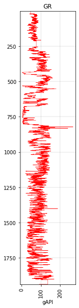
gr.plot(c='r', lw=0.5)
<AxesSubplot:title={'center':'GR'}, xlabel='gAPI'>
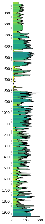
There’s also a pseudocolor 2D ribbon plot:
gr.plot_2d()
<AxesSubplot:>

You can optionally show the curve trace as well with curve=True:
gr.plot_2d(cmap='viridis_r', curve=True, lw=0.3, edgecolor='k')
plt.xlim(0,200)
(0.0, 200.0)
Despike
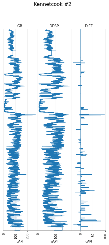
You can despike with a window length for the trend and a Z-score to clip at — the curve is compared to the median in the window using the standard deviation from the entire curve. Here’s the difference:
p129.data['DESP'] = gr.despike(z=1)
p129.data['DIFF'] = gr - p129.data['DESP']
p129.plot(tracks=['GR', 'DESP', 'DIFF'])
Blocking
We can block a curve. Let’s look at a small segment:
segment = gr.to_basis(start=600, stop=680)
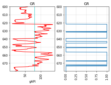
We can create a binary log (0’s and 1’s) with a simple cutoff:
fig, axs = plt.subplots(ncols=2)

# The original log on the left.
segment.plot(ax=axs[0], c='r')
axs[0].axvline(80, c='c', alpha=0.7)

# Make and plot a blocked version.
segment.block(cutoffs=80).plot(ax=axs[1])
axs[1].set_xlabel('')
Text(0.5, 0, '')
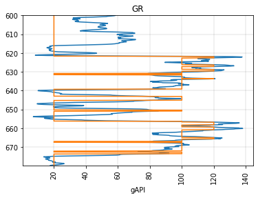
Or we can use two cutoffs and get a blocked log with three different values. By default the new values will be 0, 1, 2, but we can assign whatever we like:
fig, ax = plt.subplots()

segment.plot(ax=ax)
segment.block(cutoffs=(80, 120), values=(20, 100, 120)).plot(ax=ax)
<AxesSubplot:title={'center':'GR'}, xlabel='gAPI'>
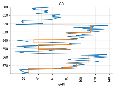
You can send a function in to determine replacement values from the original log. E.g., to replace the values with the block’s mean value:
fig, ax = plt.subplots()

segment.plot(ax=ax)
segment.block(cutoffs=80, function=np.mean).plot(ax=ax)
plt.axvline(80, color='c', lw=1)
<matplotlib.lines.Line2D at 0x7f0a8e082df0>
Instantiating a new curve
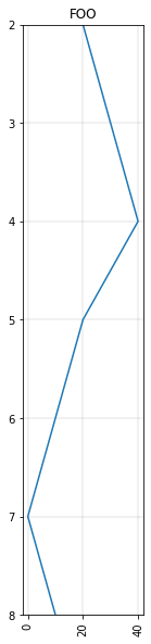
Let’s add a curve from a list of values (data) with depths (basis):
from welly import Curve

params = {'mnemonic': 'FOO', 'run':0, }
data = [20, 30, 40, 20, 10, 0, 10]
c = Curve(data, index=[2,3,4,5,6,7,8], **params)
c.plot()
<AxesSubplot:title={'center':'FOO'}>
© 2022 Agile Scientific, CC BY