Seismic attributes#

We’ll make some seismic attributes in bruges. I am going to use a very narrow 3D volume from the F3 seismic dataset (CC BY-SA 3.0) so that the dataset is not too big.

We’ll look at:

Complex trace attributes like reflection strength.
Semblance attributes.
Windowed attributes (not actually using bruges, but SciPy directly).

In general bruges is not yet directly compatible with xarray’s objects. You can always pass the internal NumPy data from an xarray.DataAarray called x like:

x.data

So it shouldn’t cause too many problems.

import numpy as np

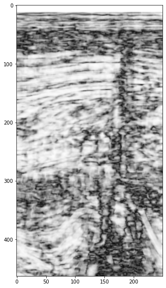
seismic = np.load('../data/F3_seismic.npy')
    
seismic.shape

(10, 250, 463)

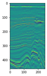
import matplotlib.pyplot as plt

plt.imshow(seismic[5].T)

<matplotlib.image.AxesImage at 0x7fd9fc865ea0>

Complex trace attributes#

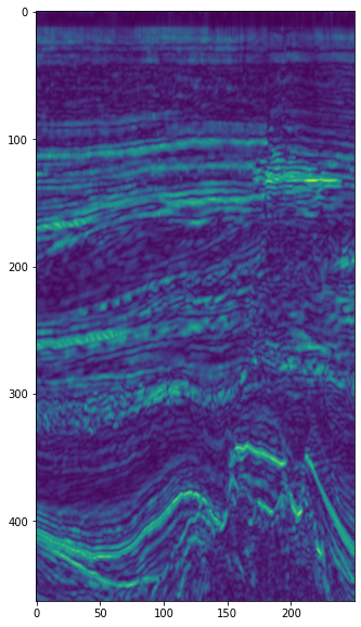
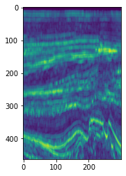
Envelope (aka reflection strength, instantaneous amplitude)#

import bruges as bg

env = bg.attribute.envelope(seismic)

plt.figure(figsize=(6, 10))
plt.imshow(env[5].T, interpolation='bicubic')

<matplotlib.image.AxesImage at 0x7fd9e7aee410>

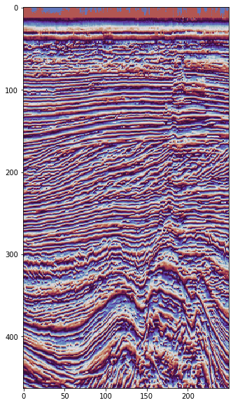
Instantaneous phase#

We’ll display this with a circular colourmap, and turn off interpolation to preven visualization artifacts.

phase = bg.attribute.instantaneous_phase(seismic)

plt.figure(figsize=(6, 10))
plt.imshow(phase[5].T, cmap='twilight_shifted', interpolation='none')

<matplotlib.image.AxesImage at 0x7fd9e7b6dab0>

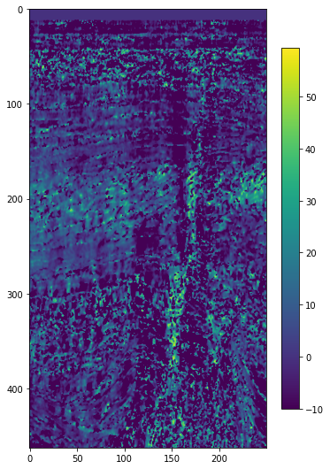
Instantaneous frequency#

freq = bg.attribute.instantaneous_frequency(seismic, dt=0.004)

plt.figure(figsize=(6, 10))
plt.imshow(freq[5].T, interpolation='bicubic', vmin=-10)
plt.colorbar(shrink=0.75)

<matplotlib.colorbar.Colorbar at 0x7fd9e79a8a90>

Similarity (family including coherency, semblance, gradient structure tensor, etc.)#

⚠️ This one takes quite a bit longer than the simpler attributes above (about a minute on my machine), so you might want to experiment on a subcube before computing the entire volume.

semb = bg.attribute.similarity(seismic, duration=0.036, dt=0.004, kind='gst')

/opt/hostedtoolcache/Python/3.10.4/x64/lib/python3.10/site-packages/bruges/attribute/discontinuity.py:77: RuntimeWarning: invalid value encountered in float_scalars
  return (eigs[0]-eigs[1]) / (eigs[0]+eigs[1])

---------------------------------------------------------------------------
KeyboardInterrupt                         Traceback (most recent call last)
Input In [6], in <cell line: 1>()
----> 1 semb = bg.attribute.similarity(seismic, duration=0.036, dt=0.004, kind='gst')

File /opt/hostedtoolcache/Python/3.10.4/x64/lib/python3.10/site-packages/bruges/attribute/discontinuity.py:124, in discontinuity(traces, duration, dt, step_out, kind, sigma)
    118 else:
    119     raise NotImplementedError("Expected 2D or 3D seismic data.")
    121 methods = {
    122     "marfurt": moving_window(traces, marfurt, window),
    123     "gersztenkorn": moving_window(traces, gersztenkorn, window),
--> 124     "gst": gst_discontinuity(traces, window, sigma)
    125 }
    127 return np.squeeze(methods[kind])

File /opt/hostedtoolcache/Python/3.10.4/x64/lib/python3.10/site-packages/bruges/attribute/discontinuity.py:89, in gst_discontinuity(seismic, window, sigma)
     81 """
     82 Gradient structure tensor discontinuity.
     83 
   (...)
     86 SEG, Expanded Abstracts, 668-671.
     87 """
     88 grad = gradients(seismic, sigma)
---> 89 return moving_window4d(grad, window, gst_calc)

File /opt/hostedtoolcache/Python/3.10.4/x64/lib/python3.10/site-packages/bruges/attribute/discontinuity.py:69, in moving_window4d(grad, window, func)
     67 for i, j, k in np.ndindex(out.shape):
     68     region = padded[i:i+window[0], j:j+window[1], k:k+window[2], :]
---> 69     out[i,j,k] = func(region)
     70 return out

File /opt/hostedtoolcache/Python/3.10.4/x64/lib/python3.10/site-packages/bruges/attribute/discontinuity.py:76, in gst_calc(region)
     74 region = region.reshape(-1, 3)
     75 gst = region.T.dot(region)
---> 76 eigs = np.sort(np.linalg.eigvalsh(gst))[::-1]
     77 return (eigs[0]-eigs[1]) / (eigs[0]+eigs[1])

File <__array_function__ internals>:180, in eigvalsh(*args, **kwargs)

File /opt/hostedtoolcache/Python/3.10.4/x64/lib/python3.10/site-packages/numpy/linalg/linalg.py:1151, in eigvalsh(a, UPLO)
   1148 if UPLO not in ('L', 'U'):
   1149     raise ValueError("UPLO argument must be 'L' or 'U'")
-> 1151 extobj = get_linalg_error_extobj(
   1152     _raise_linalgerror_eigenvalues_nonconvergence)
   1153 if UPLO == 'L':
   1154     gufunc = _umath_linalg.eigvalsh_lo

File /opt/hostedtoolcache/Python/3.10.4/x64/lib/python3.10/site-packages/numpy/linalg/linalg.py:107, in get_linalg_error_extobj(callback)
    106 def get_linalg_error_extobj(callback):
--> 107     extobj = list(_linalg_error_extobj)  # make a copy
    108     extobj[2] = callback
    109     return extobj

KeyboardInterrupt: 

plt.figure(figsize=(6, 10))
plt.imshow(semb[5].T, cmap='gray', interpolation='bicubic')

<matplotlib.image.AxesImage at 0x7f415aeb73a0>

Windowed attribute statistics#

Let’s say we’d like to compute the mean amplitude over a dataset, but inside a running window.

The easiest way to accomplish this is with scipy.ndimage.generic_filter(). It’s nice because it handles the mechanics of stepping over the array.

This wants a so-called ‘callback’ function, to which each sub-volume will be passed. Let’s see:

def rms(data):
    """
    Root mean square.
    
    Example
    >>> rms([3, 4, 5])
    4.08248290463863
    """
    data = np.asanyarray(data)
    return np.sqrt(np.sum(data**2) / data.size)

generic_filter wants the data, the function, and the size of the sub-volume to pass in to the callback function. This can be trace-by-trace (use 1 for the first two dimensions) or multi-trace (e.g. use 3). A larger template will be slower to compute of course.

from scipy.ndimage import generic_filter

seismic_rms = generic_filter(seismic, rms, size=(1, 1, 11))
seismic_rms.shape

(225, 300, 463)

The shape is the same as the original dataset. That’s convenient.

plt.imshow(seismic_rms[5].T)

<matplotlib.image.AxesImage at 0x7f79a06411c0>

Other statistics#

To get other statistics, we just need to change the function, or simply pass in a function from NumPy or wherever, eg:

seismic_median = generic_filter(seismic, np.median, size=(3, 3, 11))

Gives a median filter computed over a kernel with shape 3 × 3 inlines by crosslines, and 11 time samples.

Faster, but fiddly-er#

For the trace-by-trace case, we could speed this up by computing the RMS over various shifted versions of the seismic. This does not need more memory, because the shifted cubes are just views of the data. However, it does mean that the result will be shorter than the input, unless we somehow deal with the boundaries.

For a window of length n, we can make a set of shifted views of the volume:

n = 11
vols = [seismic[:, :, ni:ni-n] for ni in range(n)]

Then compute the RMS over this collection; on my computer this is about 200 times faster than the generic_filter approach above (900 ms vs 3 minutes):

data = np.asanyarray(vols)
seismic_rms = np.sqrt(np.sum(data**2, axis=0) / n)

Note that the result is not the same shape as the data, however:

seismic_rms.shape

(225, 300, 452)

Note that this volume has 5 samples ‘missing’ at the top, and another 5 at the bottom.

Also, this method won’t work for multi-trace statistics. So generic_filter is probably the best general approach.

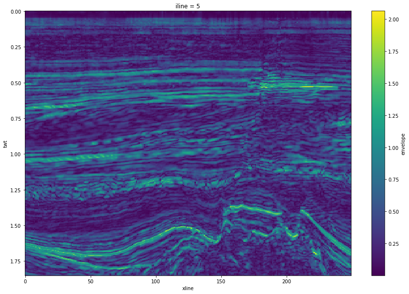
Attributes and `xarray`#

Let’s look at how to make this into an xarray.DataArray:

import xarray as xr

# I don't have the inline, xline numbers, so I'll just use the shape.
i, x, t = env.shape
iline = np.arange(i)
xline = np.arange(x)
twt = np.arange(t) * 0.004

env_xr = xr.DataArray(env,
                      name='envelope',
                      coords=[iline, xline, twt],
                      dims=['iline', 'xline', 'twt'],
                      )

This makes lots of things easier, like plotting:

plt.figure(figsize=(15, 10))
env_xr[5].T.plot.imshow(origin='upper')

<matplotlib.image.AxesImage at 0x7f18c79ab730>