Welcome to bruges

This page gives a quick look at some of the things bruges can do.

This library does all sorts of things so it’s hard to show you a single workflow and say, “here’s how to use bruges”. But making a simple wedge model will let us show you several features, and maybe it will help you see how to use bruges in your own work.

Seismic wedge models provide seismic interpreters a quantitative way of studying thin-bed stratigraphy at or below seismic resolution. Here’s the workflow:

1. Define the layer geometries.

2. Give those layers rock properties.

3. Calculate reflection coefficients.

4. Make a seismic wavelet.

5. Model the seismic response by convolving the reflectivities with the wavelet.

Let’s get started!

Make a wedge

The wedge function in models submodule allows you to generate a variety of stratigraphic geometries. The default gives us a model m which is a 2-D NumPy array of size (100, 100). It has 3 layers in it.

import bruges as bg

m, top, base, ref = bg.models.wedge(width=120)

The wedge function returns a tuple containing the model m, as well as the a top, base and ref denoting some key boundaries in the model. Let’s put these objects on a plot.

import matplotlib.pyplot as plt

plt.imshow(m)
plt.plot(top, 'r', lw=4)
plt.plot(base, 'r', lw=4)
plt.axvline(ref, c='k', ls='--')
plt.show()

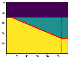
The model m is a 2-D NumPy array where each element is an index corresponding to each layer. The purple layer region has 0, the green layer has 1 and the yellow layer is 2 . top and base, shown in red, are the depths down to the “top” of wedge layer and “base” of the wedge layer respectively. ref stands for “reference trace” and it denotes the position where the wedge has a thickness factor of 1.

Make an earth

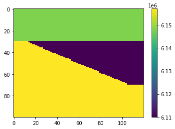
The model is filled with integers, but the earth is filled with rock properties. We need to replace those integers with rock properties.

Let’s define P-wave velocity, S-wave velocity, and rho (density) for our 3 rock types:

import numpy as np

vps = np.array([2320, 2350, 2350])
vss = np.array([1150, 1250, 1200])
rhos = np.array([2650, 2600, 2620])

We can use these to make vp and rho earth models. We can use NumPy’s fancy indexing by passing our array of indicies to access the rock properties (in this case acoustic impedance) for every element at once.

vp = vps[m]
vs = vss[m]
rho = rhos[m]

And plot the acoustic impedance to check it looks reasonable:

impedance = vp * rho

plt.imshow(impedance, interpolation='none')
plt.colorbar()
plt.show()

Acoustic reflectivity

We don’t actually need impedance, we need reflectivity. We can use bruges to create a section of normal incidence reflection coefficient; this will be what we convolve with a wavelet.

Here’s how to get the acoustic reflectivity:

rc = bg.reflection.acoustic_reflectivity(vp, rho)

plt.imshow(rc)
plt.colorbar()
plt.show()

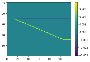
The reflections coeffients are zero almost everywhere, except at the layer boundaries. The reflection coefficient between layer 1 and layer 2 is a negative, and between layer 2 and layer 3 is a positive number. This will determine the scale and polarity of the seismic amplitudes.

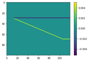
Offset reflectivity

We can also calculate the exact Zoeppritz offset reflectivity. For example, to compute the reflectivity at 10 degrees of offset — note that this results in complex numbers, so we’ll only use the real part in the plot:

rc_10 = bg.reflection.reflectivity(vp, vs, rho, theta=10)

plt.imshow(rc_10.real)
plt.colorbar()
plt.show()

As with the elastic impedance calculation, we can create a range of angles at once:

rc = bg.reflection.reflectivity(vp, vs, rho, theta=np.arange(60), method='shuey')

rc.shape

(60, 100, 120)

The 10-degree reflectivity we computed before is in there as rc[10], but we can also see how reflectivity varies with angle:

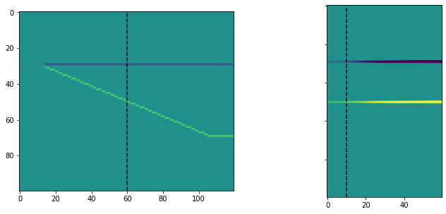
offset = 10  # degrees
trace = 60

fig, axs = plt.subplots(ncols=2, figsize=(12, 5), sharey=True)
axs[0].imshow(rc[offset].real, vmin=-0.01, vmax=0.01)
axs[0].axvline(trace, c='k', ls='--')
axs[1].imshow(rc[:, :, trace].real.T, vmin=-0.01, vmax=0.01)
axs[1].axvline(offset, c='k', ls='--')
plt.show()

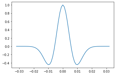
A 1D wavelet

Let’s create a Ricker wavelet to serve as our seismic pulse. We specify it has a length of 0.256 s, a sample interval of 0.002 s, and corner frequencies of 8, 12, 20, and 40 Hz:

w, t = bg.filters.ricker(0.064, 0.001, 40)

plt.plot(t, w)

[<matplotlib.lines.Line2D at 0x7f32b34715d0>]

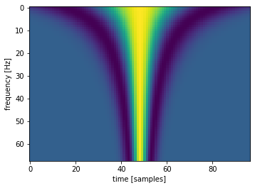
A 2D wavelet bank

There are several wavelet functions; they can all take a sequence of frequencies and produce all of them at once as a filter bank:

w_bank, t = bg.filters.ricker(0.096, 0.001, np.arange(12, 80))

plt.imshow(w_bank)
plt.xlabel('time [samples]')
plt.ylabel('frequency [Hz]')

Text(0, 0.5, 'frequency [Hz]')

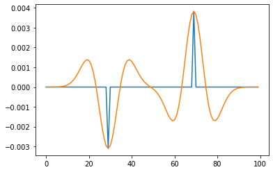
A 1D convolution

We can use bruges to perform a convolution.

Remember our RC series is 3D. Let’s keep it simple for now and look at a single waveform from the reference location ref in our model. The synthetic seismic trace is band-limited filtering of the reflectivity spikes. When these spikes get closer together the waveforms will “tune” with one another and won’t necessarily line up with the reflectivity series.

rc_ref = rc[0, :, ref]

syn = bg.filters.convolve(rc_ref, w)

plt.plot(rc_ref)
plt.plot(syn)
plt.show()

In the 1D case, it would have been easy enough to use np.convolve to do this. The equivalent code is:

syn = np.convolve(rc_ref, w, mode='same')

2D convolution

But when the reflectivity is two-dimensional (or more!), you need to use np.apply_along_axis or some other trick to essentially loop over the traces. But don’t worry! The bruges function will compute the convolution for you over all of the dimensions at once.

There’s a small catch, because of how models are organized. For plotting convenience, time is on the first axis of a model slice or profile, not the last axis (as is usual with, say, seismic data — with the result that you typically have to transpose such data for display). So we have to tell the convolve() function which is our Z (time) axis:

syn = bg.filters.convolve(rc, w, axis=1)

syn.shape

(60, 100, 120)

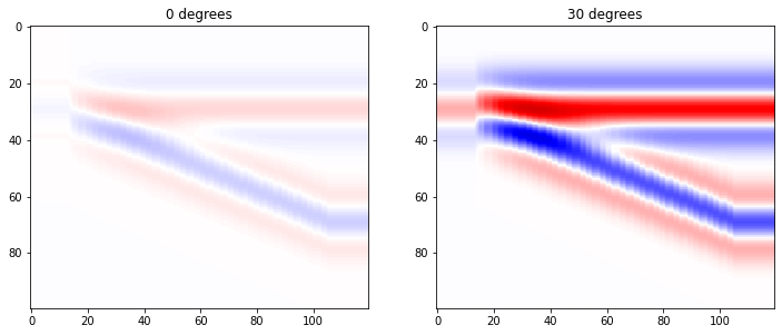
Remember those are offsets in the first dimension. Let’s look at the zero-offset synthetic alongside the 30-degree panel:

# A quick way to set a sensible max, so both panels have the same colours.
ma = np.percentile(syn, 99.9)

near, far = 0, 30

fig, axs = plt.subplots(ncols=2, figsize=(12, 5))
axs[0].imshow(syn[near], cmap='seismic_r', vmin=-ma, vmax=ma)
axs[0].set_title(f'{near} degrees')
axs[1].imshow(syn[far], cmap='seismic_r', vmin=-ma, vmax=ma)
axs[1].set_title(f'{far} degrees')
plt.show()

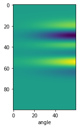
Or we could look at a single ‘angle gather’:

trace = 70

plt.imshow(syn[:, :, trace].T)
plt.xlabel('angle')

Text(0.5, 0, 'angle')

Bend your mind

The convolution function will also accept a filter bank (a collection of wavelets at different frequencies). We made one earlier called w_bank.

Watch out: the result of this convolution will be 4-dimensional!

syn = bg.filters.convolve(rc, w_bank, axis=1)

syn.shape

(68, 60, 100, 120)

Notice that the time axis has moved back to dimension 2 as a result of the wavelet having two dimensions: its frequency dimension is now in dimension 0 of the array.

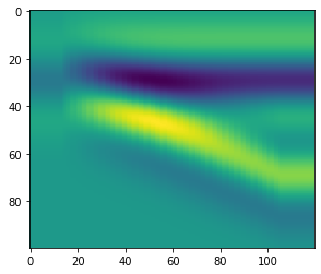
So we can look at the synthetic created with a 22 Hz wavelet (the wavelet bank started at 12 Hz, so this is slice 10 in the first dimension), and at 30 degrees of offset (slice 30 in the second dimension):

plt.imshow(syn[10, 30])

<matplotlib.image.AxesImage at 0x7f32b5a895a0>

But we could also look at how the amplitude varies in the stratigraphic middle (timeslice 50) of the thickest part of the wedge (trace ref), when we vary frequency and offset:

plt.imshow(syn[:, :, 50, ref])
plt.xlabel('offset')
plt.ylabel('frequency')

Text(0, 0.5, 'frequency')

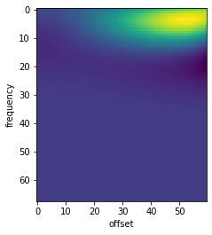
Not surprisingly, we only see amplitudes here at low frequencies (it’s the middle of the wedge). Interestingly, we also need far offsets.